2. Classifying Synthetic Sequences - The Square Model
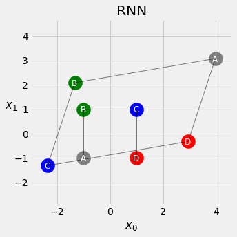
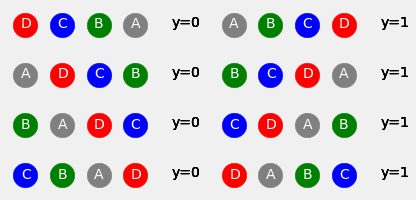
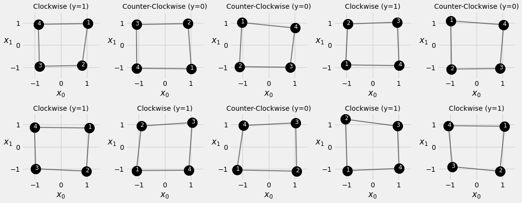
This is a simplified example of sequence modelling for classification. In this example, each sequence contains exactly four symbols, A, B, C, D, which can be ordered either clockwise or counter clockwise. Given a collection of sequences, the task is to classify if the symbols are in clockwise order (target variable \(y=1\)) or counter clockwise (target variable \(y=0\)).
The simplifications made include:
binary classification (a slightly more complex scenario is multi-class classification);
uniform sequence length, all sequences are of the same length 4, so no padding is needed;
the vocabulary size is tiny, 4 in this case;
the feature/embeding space for each symbol/token is 2 so that we can visualise in a Cartesian coordinate system. Word Embeddings are at 50+ dimensions.
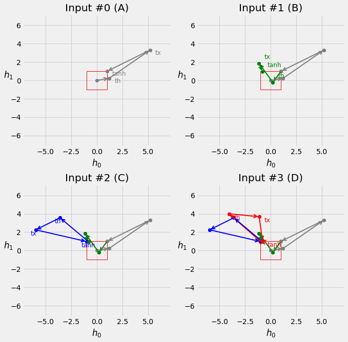
similarly for convenience of visualisation, the hidden dimension chosen is also 2.
2.1. Download Untility Files for Plotting and Data Generation
Download these utility functions first and place them in the same directory as this notebook.
from IPython.display import FileLink, FileLinks
FileLink('plots.py')
FileLink('util.py')
FileLink('replay.py')
2.2. Imports
import numpy as np

import torch
import torch.optim as optim
import torch.nn as nn
import torch.nn.functional as F

from torch.utils.data import DataLoader, Dataset, random_split, TensorDataset
from torch.nn.utils import rnn as rnn_utils
from util import StepByStep
from plots import *
2.3. Synthetic Data Generation
2.3.1. Sequence Generation Function
This function generate sequences, each of four data points, located close to a perfect square with four corners at [-1, -1], [-1, 1], [1, 1], [1, -1], respectively.
import numpy as np

def generate_sequences(n=128, variable_len=False, seed=13):
    basic_corners = np.array([[-1, -1], [-1, 1], [1, 1], [1, -1]])
    np.random.seed(seed)
    bases = np.random.randint(4, size=n)
    if variable_len:
        lengths = np.random.randint(3, size=n) + 2
    else:
        lengths = [4] * n
    directions = np.random.randint(2, size=n)
    points = [basic_corners[[(b + i) % 4 for i in range(4)]][slice(None, None, d*2-1)][:l] + np.random.randn(l, 2) * 0.1 for b, d, l in zip(bases, directions, lengths)]
    return points, directions
2.3.2. How does the sequence data look like
fig = counter_vs_clock(draw_arrows=False)
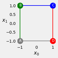
fig = counter_vs_clock()
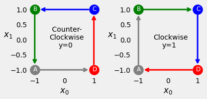
fig = plot_sequences()
points, directions = generate_sequences(n=128, seed=13)
fig = plot_data(points, directions)
2.4. Square Model
2.4.1. Dataset Preparation
test_points, test_directions = generate_sequences(seed=19)
2.4.2. Data Preparation
train_data = TensorDataset(torch.as_tensor(points).float(),
                           torch.as_tensor(directions).view(-1, 1).float())
test_data = TensorDataset(torch.as_tensor(test_points).float(),
                          torch.as_tensor(test_directions).view(-1, 1).float())

train_loader = DataLoader(train_data, batch_size=16, shuffle=True)
test_loader = DataLoader(test_data, batch_size=16)
2.4.3. Model Configuration
The SquareModel creates a single layered RNN with fully connected layer as classifier.
Your Turn
Note in the model, we did not use a sigmoid function, so what loss function should we use for binary classification?
class SquareModel(nn.Module):
    def __init__(self, n_features, hidden_dim, n_outputs):
        super(SquareModel, self).__init__()
        self.hidden_dim = hidden_dim
        self.n_features = n_features
        self.n_outputs = n_outputs
        self.hidden = None
        # Simple RNN
        self.basic_rnn = nn.RNN(self.n_features, self.hidden_dim, batch_first=True)
        # Classifier to produce as many logits as outputs
        self.classifier = nn.Linear(self.hidden_dim, self.n_outputs)

    def forward(self, X):
        # X is batch first (N, L, F)
        # output is (N, L, H)
        # final hidden state is (1, N, H)
        batch_first_output, self.hidden = self.basic_rnn(X)

        # only last item in sequence (N, 1, H)
        last_output = batch_first_output[:, -1]
        # classifier will output (N, 1, n_outputs)
        out = self.classifier(last_output)

        # final output is (N, n_outputs)
        return out.view(-1, self.n_outputs)
Tip
Note the BCEWithLogitsLoss() loss function. Modify the model and change the loss function, and see if you can still achieve the same results.
torch.manual_seed(21)
model = SquareModel(n_features=2, hidden_dim=2, n_outputs=1)
loss = nn.BCEWithLogitsLoss()
optimizer = optim.Adam(model.parameters(), lr=0.01)
2.4.4. Model Training
The StepByStep class encapsulated the training routine as well as the data loading into methods such as:
_mini_batch_make_train_step_make_val_step
You may want to take a closer look at the StepByStep in the util.py file to learn how to factorize your code into a reusable blocks.
sbs_rnn = StepByStep(model, loss, optimizer)
sbs_rnn.set_loaders(train_loader, test_loader)
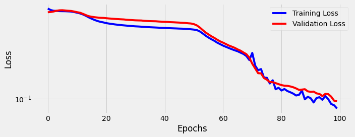
sbs_rnn.train(100)
fig = sbs_rnn.plot_losses()
StepByStep.loader_apply(test_loader, sbs_rnn.correct)
tensor([[50, 53],
        [75, 75]])