4. Sequence to Sequence Models
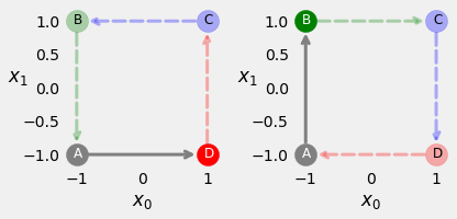
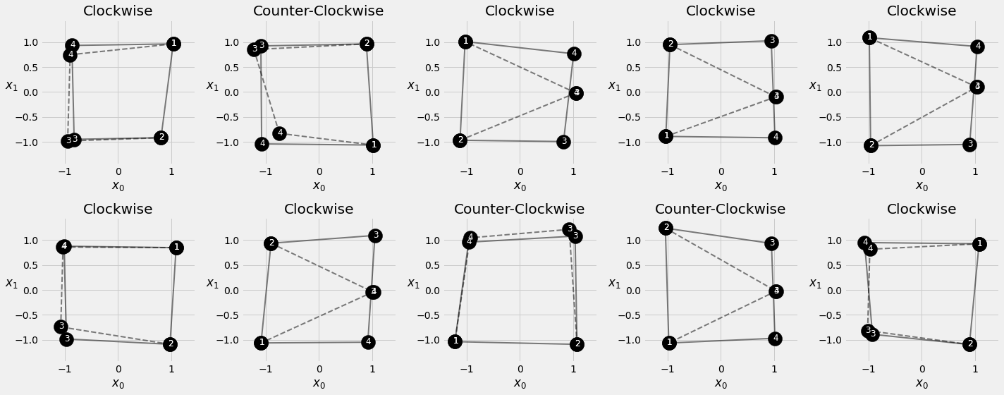
In this notebook, we will be using the same squares as before, but this time know the first two corners (the source sequence) and ask our model to predict the next two corners (the target sequence). As with every sequence-related problem, the order is important, so it is not enough to get the corner’s coordinates right, but they should follow the same direction (clockwise or counter-clockwise).
4.1. Download Plotting and Helper Functions
Download the followings files and place them in the same folder as the notebook before proceed further. These files contain the utility functions and plotting functions needed for this notebook.
from IPython.display import FileLink, FileLinks
FileLink('plots.py')
FileLink('plots_seq2seq.py')
FileLink('util.py')
FileLink('replay.py')
4.2. Imports
import copy
import numpy as np

import torch
import torch.optim as optim
import torch.nn as nn
import torch.nn.functional as F
from torch.utils.data import DataLoader, Dataset, random_split, TensorDataset
from util import StepByStep
from plots import *
from plots_seq2seq import *
4.3. Data Generation
Same method as before for generating noisy squares.
def generate_sequences(n=128, variable_len=False, seed=13):
    basic_corners = np.array([[-1, -1], [-1, 1], [1, 1], [1, -1]])
    np.random.seed(seed)
    bases = np.random.randint(4, size=n)
    if variable_len:
        lengths = np.random.randint(3, size=n) + 2
    else:
        lengths = [4] * n
    directions = np.random.randint(2, size=n)
    points = [basic_corners[[(b + i) % 4 for i in range(4)]][slice(None, None, d*2-1)][:l] + np.random.randn(l, 2) * 0.1 for b, d, l in zip(bases, directions, lengths)]
    return points, directions
Visualise an counter clock-wise perfect square and a clock-wise one.
fig = counter_vs_clock(binary=False)
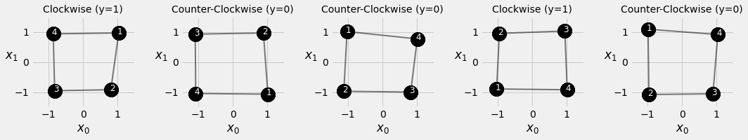
Since there are four corners to start from and two directions to follow, there are effectively eight possible sequences.
fig = plot_sequences(binary=False, target_len=2)

Generate 128 random noisy squares:
points, directions = generate_sequences(n=128, seed=13)
print(points[:2])
[array([[ 1.03487506,  0.96613817],
       [ 0.80546093, -0.91690943],
       [-0.82507582, -0.94988627],
       [-0.86696831,  0.93424827]]), array([[ 1.0184946 , -1.06510565],
       [ 0.88794931,  0.96533932],
       [-1.09113448,  0.92538647],
       [-1.07709685, -1.04139537]])]
Visualize the first five squares.
fig = plot_data(points, directions, n_rows=1)
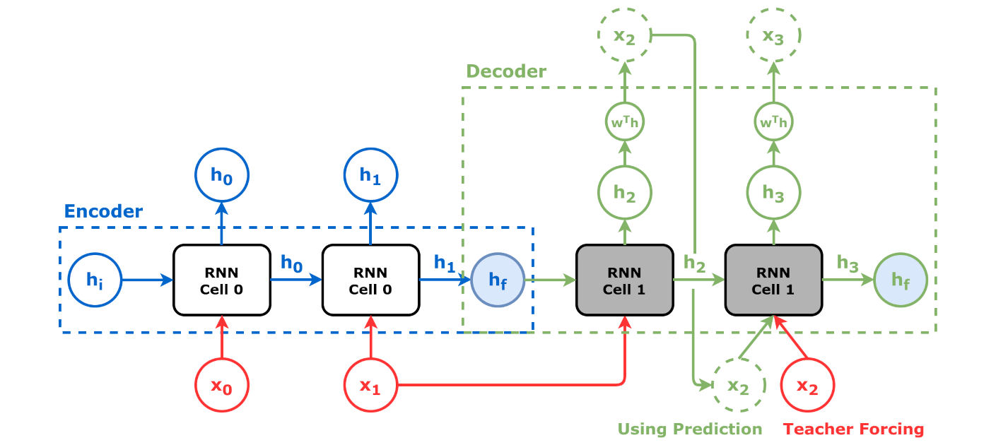
4.4. Encoder-Decoder Architecture
The encoder-decoder is a combination of two models: the encoder and the decoder.
4.4.1. Encoder
The encoder’s goal is to generate a vector representation \(\psi\) of the source sequence, that is, to encode it.
An encoder can be any of the featuriser we have seen before, e.g. a Conv1D, an Elman RNN, a GRU, an LSTM or their stacked and bidirectional variances. Here we use a GRU, \(\psi\) is the hidden state of the last cell.
Note
We kept the outputs of all cells in the Encoder code, to make the code more extendable to future “attention-based” models.
class Encoder(nn.Module):
    def __init__(self, n_features, hidden_dim):
        super().__init__()
        self.hidden_dim = hidden_dim
        self.n_features = n_features
        self.hidden = None
        self.basic_rnn = nn.GRU(self.n_features, self.hidden_dim, batch_first=True)

    def forward(self, X):
        rnn_out, self.hidden = self.basic_rnn(X)

        return rnn_out # N, L, F
A perfect square with two corners as source, and two coners target.
full_seq = torch.tensor([[-1, -1], [-1, 1], [1, 1], [1, -1]]).float().view(1, 4, 2)
source_seq = full_seq[:, :2] # first two corners
target_seq = full_seq[:, 2:] # last two corners
We use the un-trained Encoder to encode the source sequence. If trained the output vector is expected to caputre the source seqence’s intrinsic positional thus directional information.
torch.manual_seed(21)
encoder = Encoder(n_features=2, hidden_dim=2)
hidden_seq = encoder(source_seq) # output is N, L, F
hidden_final = hidden_seq[:, -1:]   # takes last hidden state
hidden_final
tensor([[[ 0.3105, -0.5263]]], grad_fn=<SliceBackward>)
# 1 training sample, N=1;
# Sequence contain two corners, Length L=2;
# Each corner is in two dimensional space, Feature F=2;
print(hidden_seq)
tensor([[[ 0.0832, -0.0356],
         [ 0.3105, -0.5263]]], grad_fn=<TransposeBackward1>)
hidden_seq[:, -1:, :]
tensor([[[ 0.3105, -0.5263]]], grad_fn=<SliceBackward>)
4.4.2. Decoder
The decoder’s goal is to generate the target sequence from an initial representation, that is, to decode it.
Very often the decorder takes the encoder’s output of last cell, as its initial hidden state, and use last input the encoder as its first input, to generate a sequence of desired length. The output of each cell through a linear transformantion (regression) to obtain the output sequence of the decoder So the encoder can be realised through an RNN or its variants as well.
The code below uses a GRU layer as a decoder.
Note
Since we are generating numerical values that represent the coordinates of the corners, we are dealing with a regression problem. So in the later model training, we use MSE as loss function.
class Decoder(nn.Module):
    def __init__(self, n_features, hidden_dim):
        super().__init__()
        self.hidden_dim = hidden_dim
        self.n_features = n_features
        self.hidden = None
        self.basic_rnn = nn.GRU(self.n_features, self.hidden_dim, batch_first=True)
        self.regression = nn.Linear(self.hidden_dim, self.n_features)

    def init_hidden(self, hidden_seq):
        # We only need the final hidden state
        hidden_final = hidden_seq[:, -1:] # N, 1, H
        # But we need to make it sequence-first
        self.hidden = hidden_final.permute(1, 0, 2) # 1, N, H

    def forward(self, X):
        # X is N, 1, F
        batch_first_output, self.hidden = self.basic_rnn(X, self.hidden)

        last_output = batch_first_output[:, -1:]
        out = self.regression(last_output)

        # N, 1, F
        return out.view(-1, 1, self.n_features)
Decoder is often considered as a generator. Here the decoder is intialised with the last hidden state of the encoder first. The initial input is the last element of the source sequence. Then it takes the previous cell output as input, in a for loop, until it generate a specified number (target sequence length) of elements.
torch.manual_seed(21)
decoder = Decoder(n_features=2, hidden_dim=2)

# Initial hidden state will be encoder's final hidden state
decoder.init_hidden(hidden_seq)
# Initial data point is the last element of source sequence
inputs = source_seq[:, -1:]

target_len = 2
for i in range(target_len):
    print(f'Hidden: {decoder.hidden}')
    out = decoder(inputs)   # Predicts coordinates
    print(f'Output: {out}\n')
    # Predicted coordinates are next step's inputs
    inputs = out
Hidden: tensor([[[ 0.3105, -0.5263]]], grad_fn=<PermuteBackward>)
Output: tensor([[[-0.2339,  0.4702]]], grad_fn=<ViewBackward>)

Hidden: tensor([[[ 0.3913, -0.6853]]], grad_fn=<StackBackward>)
Output: tensor([[[-0.0226,  0.4628]]], grad_fn=<ViewBackward>)
4.4.2.1. Teacher Forcing
There is one problem with the approach above, an untrained model will make really bad predictions, and these predictions will still be used as inputs for subsequent steps. This makes model training unnecessarily hard because the prediction error in one step is caused by both the (untrained) model and the prediction error in the previous step.
Tip
We can use the actual target sequence instead! This technique is called teacher forcing. We can ignore the predictions and use the real data from the target sequence instead.
# Initial hidden state will be encoder's final hidden state
decoder.init_hidden(hidden_seq)
# Initial data point is the last element of source sequence
inputs = source_seq[:, -1:]

target_len = 2
for i in range(target_len):
    print(f'Hidden: {decoder.hidden}')
    out = decoder(inputs) # Predicts coordinates
    print(f'Output: {out}\n')
    # But completely ignores the predictions and uses real data instead
    inputs = target_seq[:, i:i+1]
Hidden: tensor([[[ 0.3105, -0.5263]]], grad_fn=<PermuteBackward>)
Output: tensor([[[-0.2339,  0.4702]]], grad_fn=<ViewBackward>)

Hidden: tensor([[[ 0.3913, -0.6853]]], grad_fn=<StackBackward>)
Output: tensor([[[0.2265, 0.4529]]], grad_fn=<ViewBackward>)
Put the two cases together:
# Initial hidden state is encoder's final hidden state
decoder.init_hidden(hidden_seq)
# Initial data point is the last element of source sequence
inputs = source_seq[:, -1:]

teacher_forcing_prob = 0.5
target_len = 2
for i in range(target_len):
    print(f'Hidden: {decoder.hidden}')
    out = decoder(inputs)
    print(f'Output: {out}\n')
    # If it is teacher forcing
    if torch.rand(1) <= teacher_forcing_prob:
        # Takes the actual element
        inputs = target_seq[:, i:i+1]
    else:
        # Otherwise uses the last predicted output
        inputs = out
Hidden: tensor([[[ 0.3105, -0.5263]]], grad_fn=<PermuteBackward>)
Output: tensor([[[-0.2339,  0.4702]]], grad_fn=<ViewBackward>)

Hidden: tensor([[[ 0.3913, -0.6853]]], grad_fn=<StackBackward>)
Output: tensor([[[-0.0226,  0.4628]]], grad_fn=<ViewBackward>)
4.4.3. Encoder + Decoder
We can assemble a boilerplate that integrates a encoder and a decoder. Given an encoder and a decoder model, the code below implements a forward method that splits the input into the source and target sequences, loops over the generation of the target sequence, and implements teacher forcing in training mode.
class EncoderDecoder(nn.Module):
    def __init__(self, encoder, decoder, input_len, target_len, teacher_forcing_prob=0.5):
        super().__init__()
        self.encoder = encoder
        self.decoder = decoder
        self.input_len = input_len
        self.target_len = target_len
        self.teacher_forcing_prob = teacher_forcing_prob
        self.outputs = None

    def init_outputs(self, batch_size):
        device = next(self.parameters()).device
        # N, L (target), F
        self.outputs = torch.zeros(batch_size,
                              self.target_len,
                              self.encoder.n_features).to(device)

    def store_output(self, i, out):
        # Stores the output
        self.outputs[:, i:i+1, :] = out

    def forward(self, X):
        # splits the data in source and target sequences
        # the target seq will be empty in testing mode
        # N, L, F
        source_seq = X[:, :self.input_len, :]
        target_seq = X[:, self.input_len:, :]
        self.init_outputs(X.shape[0])

        # Encoder expected N, L, F
        hidden_seq = self.encoder(source_seq)
        # Output is N, L, H
        self.decoder.init_hidden(hidden_seq)

        # The last input of the encoder is also
        # the first input of the decoder
        dec_inputs = source_seq[:, -1:, :]

        # Generates as many outputs as the target length
        for i in range(self.target_len):
            # Output of decoder is N, 1, F
            out = self.decoder(dec_inputs)
            self.store_output(i, out)

            prob = self.teacher_forcing_prob
            # In evaluation/test the target sequence is
            # unknown, so we cannot use teacher forcing
            if not self.training:
                prob = 0

            # If it is teacher forcing
            if torch.rand(1) <= prob:
                # Takes the actual element
                dec_inputs = target_seq[:, i:i+1, :]
            else:
                # Otherwise uses the last predicted output
                dec_inputs = out

        return self.outputs
encdec = EncoderDecoder(encoder, decoder, input_len=2, target_len=2, teacher_forcing_prob=1.0)
encdec.train()
encdec(full_seq)
tensor([[[-0.2339,  0.4702],
         [ 0.2265,  0.4529]]], grad_fn=<CopySlices>)
encdec.eval()
encdec(source_seq)
tensor([[[-0.2339,  0.4702],
         [-0.0226,  0.4628]]], grad_fn=<CopySlices>)
4.4.4. Data Preparation
The first two corners of the square data[:, :2] are the source sequences; the last two corners data[:, 2:] are the target sequences.
points, directions = generate_sequences()
full_train = torch.as_tensor(points).float()
target_train = full_train[:, 2:]
test_points, test_directions = generate_sequences(seed=19)
full_test = torch.as_tensor(points).float()
source_test = full_test[:, :2]
target_test = full_test[:, 2:]
train_data = TensorDataset(full_train, target_train)
test_data = TensorDataset(source_test, target_test)

generator = torch.Generator()
train_loader = DataLoader(train_data, batch_size=16, shuffle=True, generator=generator)
test_loader = DataLoader(test_data, batch_size=16)
4.4.5. Model Training & Configuration
torch.manual_seed(23)
encoder = Encoder(n_features=2, hidden_dim=2)
decoder = Decoder(n_features=2, hidden_dim=2)
model = EncoderDecoder(encoder, decoder, input_len=2, target_len=2, teacher_forcing_prob=0.5)
loss = nn.MSELoss()
optimizer = optim.Adam(model.parameters(), lr=0.01)
sbs_seq = StepByStep(model, loss, optimizer)
sbs_seq.set_loaders(train_loader, test_loader)
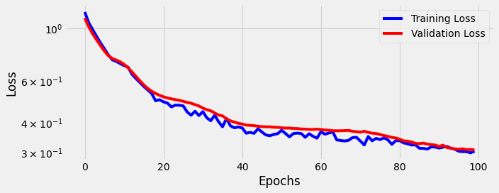
sbs_seq.train(100)
fig = sbs_seq.plot_losses()
4.4.6. Visualizing Predictions
fig = sequence_pred(sbs_seq, full_test, test_directions)
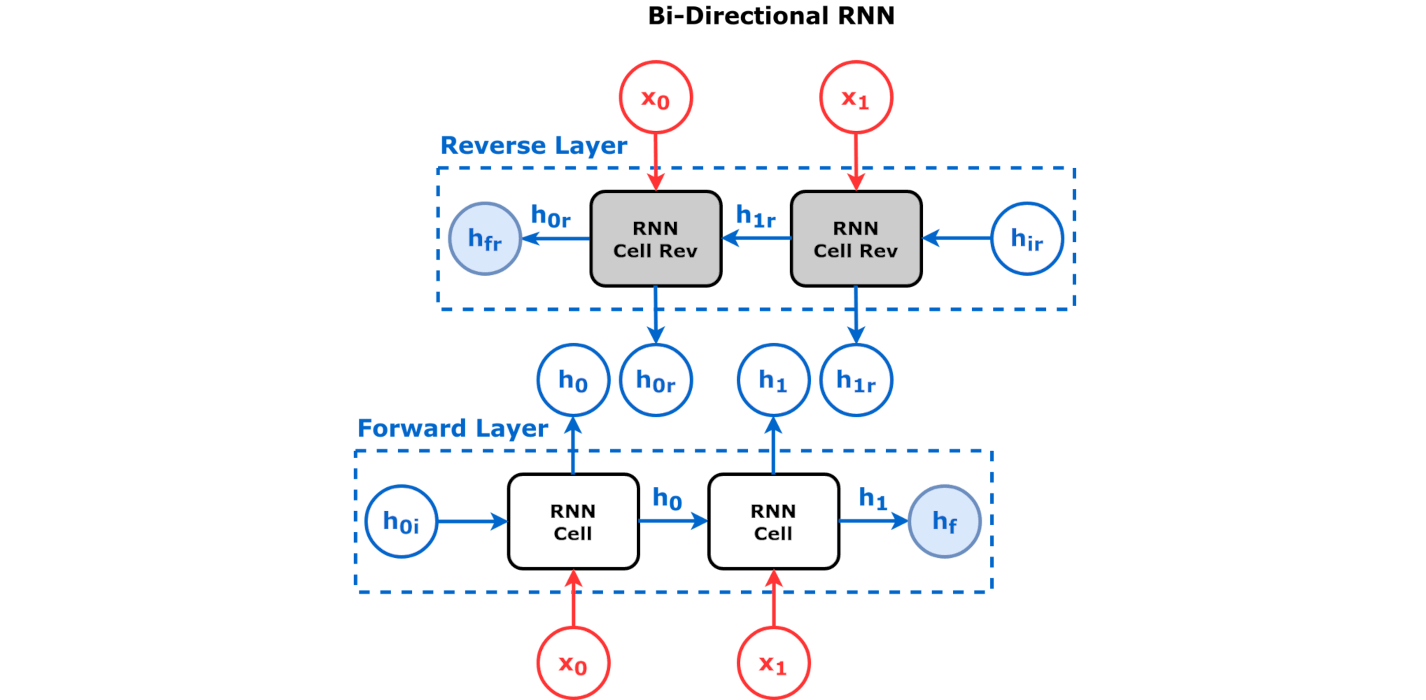
4.5. Bidirectional LSTM as an Encoder
We have been using the output of GRU above to exact the last hidden state as the representation vector \(\psi\) betwen the encoder and decoder. Note that despite the output and hidden state of a GRU cell is the same, we still used the output, rather than the hidden state. This is because the bidirectional variations outputs are hidden states are not the same. Recall that the overall output of the bidirectional RNN must have two elements:
a concatenation side-by-side of both sequences of hidden states (input aligned)
the concatenation of final hidden states of both layers, the last of the forward layer is corresponding to the last element of the sequence, the last of the backward layer is corresponding to the first element of the sequence (i.e. not input aligned).
See the figure below for clarification.
For Sequence to Sequence model, we will need an input aligned output, so the code above largely should still work (the dimenionality changed though), but conceptually we need to be clear of what’s happening.
Your Turn
Change the code above to use BiLSTM as an encoder.