1. Gated Recurrent Units (GRUs)¶

GRU addressed two fundamental limitations of Elman RNN, by introducing

Update Gate: Weights between old and new (candidate) hidden state

Update Gate

\(\begin{align*} h_{new} &= tanh(t_h+t_x) \\ h' &= h_{new} * (1 - z) + h_{old} * z \end{align*}\)

Reset Gate: Weights between input and hidden state

Reset Gate

\(h_{new} = tanh(r*t_h + t_x)\)

Both gates can be learned through linear layer followed by sigmoid to ensure they are values in the range [0,1]. Put them together, we have a GRU cell.

GRU Cell

\(h' = tanh(r*t_h + t_x) * (1-z) + h*z\)

GRU Cell

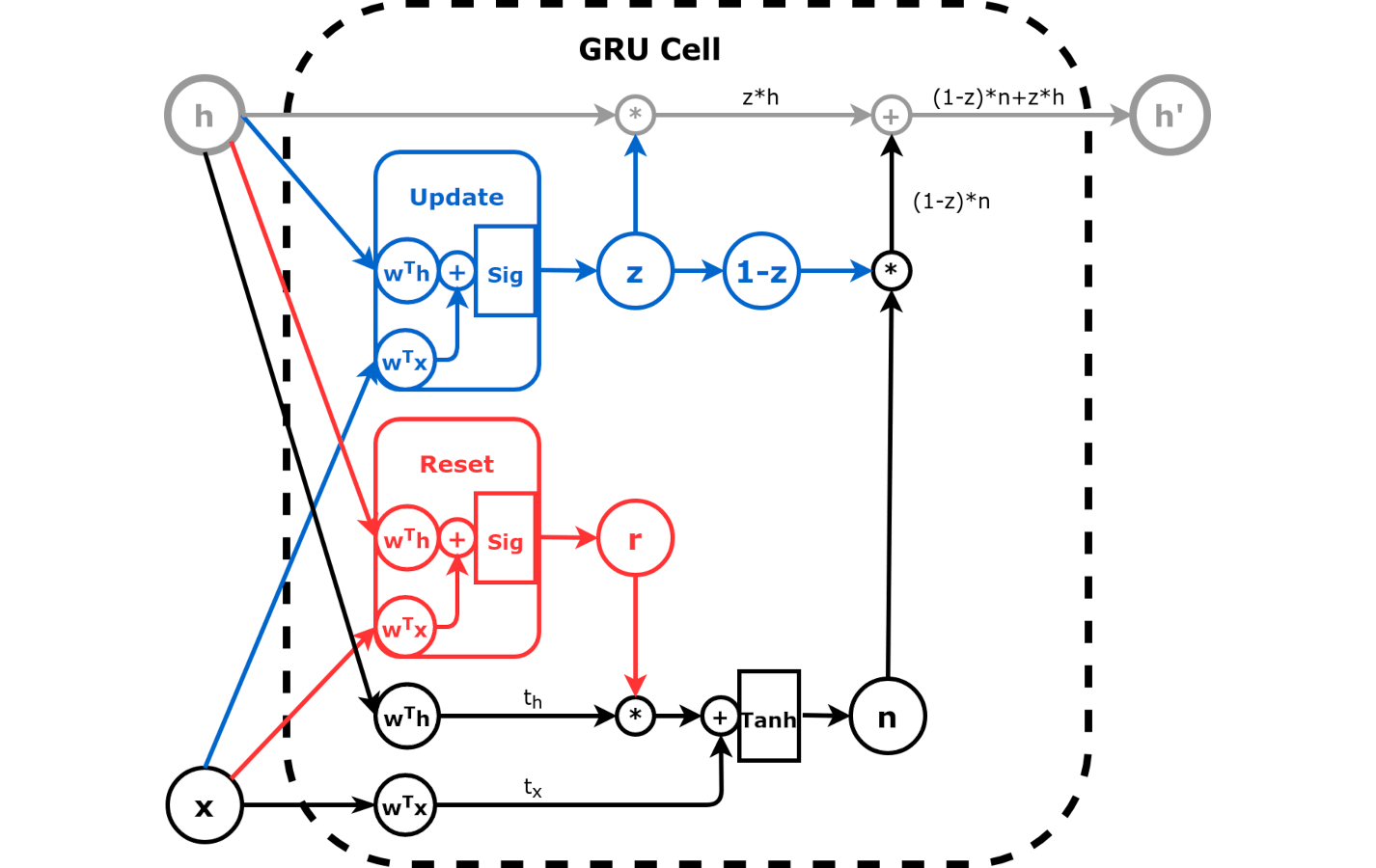
1.1. GRU Cell¶

RNN is a special case of GRU when \(r=1\) and \(z=0\).

\[\begin{split}\begin{align*} RNN: h'&=tanh(t_h+t_x) \\ GRU: h'&=\underbrace{\underbrace{tanh(\color{red}{r}*t_{hn}+t_{xn})}_{n}*\color{#0066CC}{(1-z)} + \color{gray}{h}*\color{#0066CC}{z}}_{weighted\ average\ of\ n\ and\ h} \end{align*}\end{split}\]

\[\begin{split} \begin{align*} \color{red}{r(reset\ gate)} &\color{red}{=\sigma(t_{hr}+t_{xr})} \\ \color{#0066CC}{z(update\ gate)} &\color{#0066CC}{=\sigma(t_{hz}+t_{xz})} \\ \color{black}{n (hidden\ state)}&\color{black}{=tanh(t_{hn}+t_{xn})} \end{align*} \end{split}\]

\[\begin{split} \begin{align*} \color{red}{r\ (hidden)}&\color{red}{:t_{hr}}&\color{red}{=}&\color{red}{W_{hr}}&\color{red}{h}&\color{red}{+}&\color{red}{b_{hr}} \\ \color{red}{r\ (input)}&\color{red}{:t_{xr}}&\color{red}{=}&\color{red}{W_{ir}}&\color{red}{x}&\color{red}{+}&\color{red}{b_{ir}} \\ \color{#0066CC}{z\ (hidden)}&\color{#0066CC}{:t_{hz}}&\color{#0066CC}{=}&\color{#0066CC}{W_{hz}}&\color{#0066CC}{h}&\color{#0066CC}{+}&\color{#0066CC}{b_{hz}} \\ \color{#0066CC}{z\ (input)}&\color{#0066CC}{:t_{xz}}&\color{#0066CC}{=}&\color{#0066CC}{W_{iz}}&\color{#0066CC}{x}&\color{#0066CC}{+}&\color{#0066CC}{b_{iz}} \\ n\ (hidden)&:t_{hn}& = &W_{hn}&h&+&b_{hn} \\ n\ (input)&:t_{xn}& = &W_{in}&x&+&b_{in} \end{align*} \end{split}\]

To really understand the flow of information inside the GRU cell, I suggest you try these exercises:

first, learn to look past (or literally ignore) the internals of the gates: both r and z are simply values between zero and one (for each hidden dimension)
pretend r=1; can you see that the resulting n is equivalent to the output of a simple RNN?
keep r=1 and now pretend z=0; can you see that the new hidden state h' is equivalent to the output of a simple RNN?
now pretend z=1; can you see that the new hidden state h' is simply a copy of the old hidden state (in other words, the data (x) does not have any effect)?
if you decrease r all the way to zero, the resulting n is less and less influenced by the old hidden state
if you decrease z all the way to zero, the new hidden state h' is closer and closer to n
for r=0 and z=0, the cell becomes equivalent to a linear layer followed by a Tanh activation function (in other words, the old hidden state (h) does not have any effect)

1.2. Imports¶

import numpy as np

import torch
import torch.optim as optim
import torch.nn as nn
import torch.nn.functional as F

from torch.utils.data import DataLoader, Dataset, random_split, TensorDataset
from torch.nn.utils import rnn as rnn_utils

1.3. GRU Cell¶

n_features = 2 
hidden_dim = 2
torch.manual_seed(17) 
gru_cell = nn.GRUCell(input_size=n_features, hidden_size=hidden_dim) 
gru_state = gru_cell.state_dict()
gru_state

OrderedDict([('weight_ih',
              tensor([[-0.0930,  0.0497],
                      [ 0.4670, -0.5319],
                      [-0.6656,  0.0699],
                      [-0.1662,  0.0654],
                      [-0.0449, -0.6828],
                      [-0.6769, -0.1889]])),
             ('weight_hh',
              tensor([[-0.4167, -0.4352],
                      [-0.2060, -0.3989],
                      [-0.7070, -0.5083],
                      [ 0.1418,  0.0930],
                      [-0.5729, -0.5700],
                      [-0.1818, -0.6691]])),
             ('bias_ih',
              tensor([-0.4316,  0.4019,  0.1222, -0.4647, -0.5578,  0.4493])),
             ('bias_hh',
              tensor([-0.6800,  0.4422, -0.3559, -0.0279,  0.6553,  0.2918]))])

Wi, bi = gru_state['weight_ih'], gru_state['bias_ih'] 
Wh, bh = gru_state['weight_hh'], gru_state['bias_hh']
print(Wi.shape, Wh.shape)
print(bi.shape, bh.shape)

torch.Size([6, 2]) torch.Size([6, 2])
torch.Size([6]) torch.Size([6])

1.3.1. Splitting up the `weight_ih` as an example¶

GRU Cell State Split

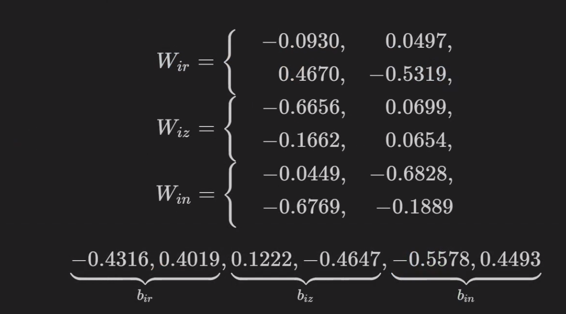
Wir, Wiz, Win = Wi.split(hidden_dim, dim=0) 
bir, biz, bin = bi.split(hidden_dim, dim=0)
Whr, Whz, Whn = Wh.split(hidden_dim, dim=0) 
bhr, bhz, bhn = bh.split(hidden_dim, dim=0)
Wxr, bxr

(tensor([[-0.0930,  0.0497],
         [ 0.4670, -0.5319]]),
 tensor([-0.4316,  0.4019]))

1.4. Creating the Linear Layers¶

We can use the weights and biases to create the corresponding linear layers:

def linear_layers(Wi, bi, Wh, bh):
    hidden_dim, n_features = Wi.size()    
    lin_input = nn.Linear(n_features, hidden_dim)
    lin_input.load_state_dict({'weight': Wi, 'bias': bi})
    lin_hidden = nn.Linear(hidden_dim, hidden_dim)
    lin_hidden.load_state_dict({'weight': Wh, 'bias': bh})
    return lin_hidden, lin_input

# reset gate - red
r_hidden, r_input = linear_layers(Wir, bir, Whr, bhr) 
# update gate - blue
z_hidden, z_input = linear_layers(Wiz, biz, Whz, bhz) 
# candidate state - black
n_hidden, n_input = linear_layers(Win, bin, Whn, bhn) 

def reset_gate(h, x):
    thr = r_hidden(h)
    txr = r_input(x)
    r = torch.sigmoid(thr + txr)
    return r  # red
    
def update_gate(h, x):
    thz = z_hidden(h)
    txz = z_input(x)
    z = torch.sigmoid(thz + txz)
    return z  # blue
    
def candidate_n(h, x, r):
    thn = n_hidden(h)
    txn = n_input(x)
    n = torch.tanh(r * thn + txn)
    return n  # black

1.5. Data Generation¶

def generate_sequences(n=128, variable_len=False, seed=13):
    basic_corners = np.array([[-1, -1], [-1, 1], [1, 1], [1, -1]])
    np.random.seed(seed)
    bases = np.random.randint(4, size=n)
    if variable_len:
        lengths = np.random.randint(3, size=n) + 2
    else:
        lengths = [4] * n
    directions = np.random.randint(2, size=n)
    points = [basic_corners[[(b + i) % 4 for i in range(4)]][slice(None, None, d*2-1)][:l] + np.random.randn(l, 2) * 0.1 for b, d, l in zip(bases, directions, lengths)]
    return points, directions

points, directions = generate_sequences(n=128, seed=13)

initial_hidden = torch.zeros(1, hidden_dim)
X = torch.as_tensor(points[0]).float()
first_corner = X[0:1]

r = reset_gate(initial_hidden, first_corner)
r

tensor([[0.2387, 0.6928]], grad_fn=<SigmoidBackward>)

Important

The reset gate scales each hidden dimension independently. It can completely suppress the values from one of the hidden dimensions while letting the other pass unchallenged. In geometrical terms, it means that the hidden space may shrink in one direction while stretching in the other.

z = update_gate(initial_hidden, first_corner)
z

tensor([[0.2984, 0.3540]], grad_fn=<SigmoidBackward>)

The reset gate is an input for the candidate hidden state (n)

n = candidate_n(initial_hidden, first_corner, r)
n

tensor([[-0.8032, -0.2275]], grad_fn=<TanhBackward>)

The update gate is telling us to keep 29.84% of the first and 35.40% of the second dimensions of the initial hidden state. The remaining 60.16% and 64.6%, respectively, are coming from the candidate hidden state (n).

h_prime = n*(1-z) + initial_hidden*z
h_prime

tensor([[-0.5635, -0.1470]], grad_fn=<AddBackward0>)

1.5.1. Verify against GRU Cell¶

We can see the nn.GRUCell() had encapsulated all the above steps. Effectively, a GRU consists of six linear layers, with

four of them require sigmoid action to learn
- two reset gates, each for hidden state and input respectively, and
- two update gates, each for hidden state and input respectively
two require tanh() activation for learning the new candidate hidden state.

gru_cell(first_corner)

tensor([[-0.5635, -0.1470]], grad_fn=<AddBackward0>)

CITS4012 Natural Language Processing