2. Long Short Term Memories (LSTMs)
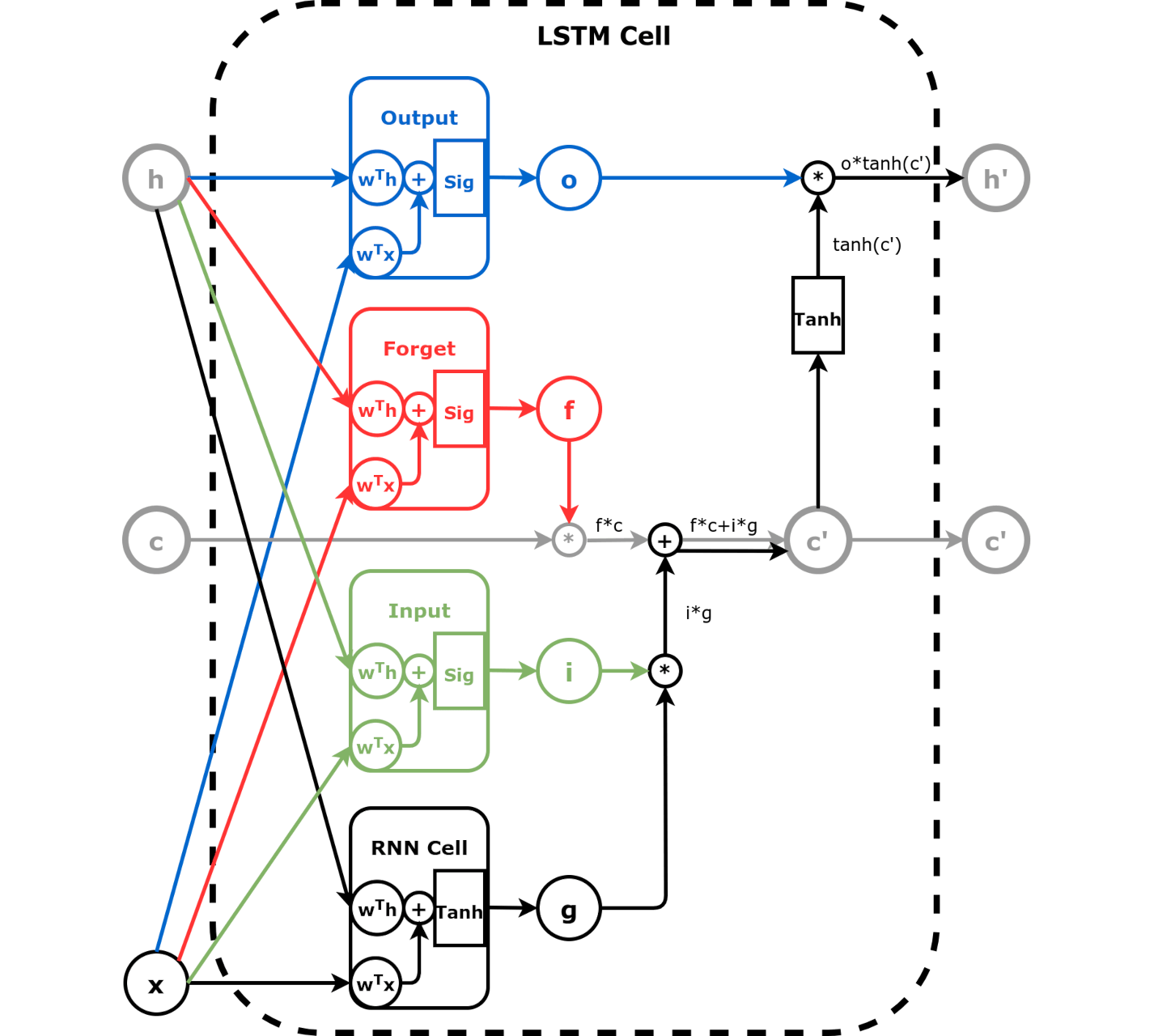
In addtion to the bounded hidden state (between [-1,1]), LSTM introduced an unbounded cell state, which is mimic the “long term memory”. This allows more past information to be kept and thus passed to the current cell, because the gradient is not squashed to approach zero as fast as tanh, so it is also refered to as a “gradient highway”. In contrast, the hidden state keeps more recent information, thus responsible for the “short term memory”.
The candidate hidden state
Cell state is an unbounded weighted sum of the candidate hidden state \(g\) and previous cell state \(c\), weighted by learnt input gate \(i\) and forget gate \(f\), respectively.
The new cell state
The new hidden state is obtained by bounding the new cell state (\(c'\)) before applying output gate weights (\(o\))
The new hidden state
2.1. Imports
import numpy as np

import torch
import torch.optim as optim
import torch.nn as nn
import torch.nn.functional as F

from torch.utils.data import DataLoader, Dataset, random_split, TensorDataset
from torch.nn.utils import rnn as rnn_utils
2.2. LSTM Cell
There are two sets of weights for each type of gates, one for hidden state, one for input. They are learnt through a linear layer followed by sigmoid like in a GRU cell.
2.2.1. nn.LSTMCell
Let’s take a look at the weights generated by nn.LSTMCell.
n_features = 2
hidden_dim = 2

torch.manual_seed(17)
lstm_cell = nn.LSTMCell(input_size=n_features, hidden_size=hidden_dim)
lstm_state = lstm_cell.state_dict()
lstm_state
OrderedDict([('weight_ih',
              tensor([[-0.0930,  0.0497],
                      [ 0.4670, -0.5319],
                      [-0.6656,  0.0699],
                      [-0.1662,  0.0654],
                      [-0.0449, -0.6828],
                      [-0.6769, -0.1889],
                      [-0.4167, -0.4352],
                      [-0.2060, -0.3989]])),
             ('weight_hh',
              tensor([[-0.7070, -0.5083],
                      [ 0.1418,  0.0930],
                      [-0.5729, -0.5700],
                      [-0.1818, -0.6691],
                      [-0.4316,  0.4019],
                      [ 0.1222, -0.4647],
                      [-0.5578,  0.4493],
                      [-0.6800,  0.4422]])),
             ('bias_ih',
              tensor([-0.3559, -0.0279,  0.6553,  0.2918,  0.4007,  0.3262, -0.0778, -0.3002])),
             ('bias_hh',
              tensor([-0.3991, -0.3200,  0.3483, -0.2604, -0.1582,  0.5558,  0.5761, -0.3919]))])
2.2.2. Replicate a LSTMCell Manually
The code below tries to use the above the weights, manually create the linear layers for learning the gates.
def linear_layers(Wi, bi, Wh, bh):
    hidden_dim, n_features = Wi.size()
    lin_input = nn.Linear(n_features, hidden_dim)
    lin_input.load_state_dict({'weight': Wi, 'bias': bi})
    lin_hidden = nn.Linear(hidden_dim, hidden_dim)
    lin_hidden.load_state_dict({'weight': Wh, 'bias': bh})
    return lin_hidden, lin_input
Split the weights and the create the linear layers for input, forget and output gate. Note the candidate hidden state is an Elman RNN.
Wx, bx = lstm_state['weight_ih'], lstm_state['bias_ih']
Wh, bh = lstm_state['weight_hh'], lstm_state['bias_hh']

# Split weights and biases for data points
Wxi, Wxf, Wxg, Wxo = Wx.split(hidden_dim, dim=0)
bxi, bxf, bxg, bxo = bx.split(hidden_dim, dim=0)
# Split weights and biases for hidden state
Whi, Whf, Whg, Who = Wh.split(hidden_dim, dim=0)
bhi, bhf, bhg, bho = bh.split(hidden_dim, dim=0)

# Creates linear layers for the components
i_hidden, i_input = linear_layers(Wxi, bxi, Whi, bhi) # input gate - green
f_hidden, f_input = linear_layers(Wxf, bxf, Whf, bhf) # forget gate - red
o_hidden, o_input = linear_layers(Wxo, bxo, Who, bho) # output gate - blue
g_cell = nn.RNNCell(n_features, hidden_dim) # black
g_cell.load_state_dict({'weight_ih': Wxg, 'bias_ih': bxg,
                        'weight_hh': Whg, 'bias_hh': bhg})
<All keys matched successfully>
def forget_gate(h, x):
    thf = f_hidden(h)
    txf = f_input(x)
    f = torch.sigmoid(thf + txf)
    return f  # red

def output_gate(h, x):
    tho = o_hidden(h)
    txo = o_input(x)
    o = torch.sigmoid(tho + txo)
    return o  # blue

def input_gate(h, x):
    thi = i_hidden(h)
    txi = i_input(x)
    i = torch.sigmoid(thi + txi)
    return i  # green
2.2.3. Data Generation
Same square sequence is used here to verify that our manual LSTM produces the same result as nn.LSTMCell.
def generate_sequences(n=128, variable_len=False, seed=13):
    basic_corners = np.array([[-1, -1], [-1, 1], [1, 1], [1, -1]])
    np.random.seed(seed)
    bases = np.random.randint(4, size=n)
    if variable_len:
        lengths = np.random.randint(3, size=n) + 2
    else:
        lengths = [4] * n
    directions = np.random.randint(2, size=n)
    points = [basic_corners[[(b + i) % 4 for i in range(4)]][slice(None, None, d*2-1)][:l] + np.random.randn(l, 2) * 0.1 for b, d, l in zip(bases, directions, lengths)]
    return points, directions
points, directions = generate_sequences(n=128, seed=13)
initial_hidden = torch.zeros(1, hidden_dim)
initial_cell = torch.zeros(1, hidden_dim)

X = torch.as_tensor(points[0]).float()
first_corner = X[0:1]
g = g_cell(first_corner)
i = input_gate(initial_hidden, first_corner)
gated_input = g * i
gated_input
tensor([[-0.1340, -0.0004]], grad_fn=<MulBackward0>)
f = forget_gate(initial_hidden, first_corner)
gated_cell = initial_cell * f
gated_cell
tensor([[0., 0.]], grad_fn=<MulBackward0>)
c_prime = gated_cell + gated_input
c_prime
tensor([[-0.1340, -0.0004]], grad_fn=<AddBackward0>)
o = output_gate(initial_hidden, first_corner)
h_prime = o * torch.tanh(c_prime)
h_prime
tensor([[-5.4936e-02, -8.3810e-05]], grad_fn=<MulBackward0>)
LSTM Cell output hidden state and cell state.
(h_prime, c_prime)
(tensor([[-5.4936e-02, -8.3810e-05]], grad_fn=<MulBackward0>),
 tensor([[-0.1340, -0.0004]], grad_fn=<AddBackward0>))
2.2.4. Verify the result against nn.LSTMCell
lstm_cell(first_corner)
(tensor([[-5.4936e-02, -8.3810e-05]], grad_fn=<MulBackward0>),
 tensor([[-0.1340, -0.0004]], grad_fn=<AddBackward0>))
BiLSTM Layer
Find out how to create a Bidirectional LSTM Layer in PyTorch? What’s the output look like?