4. Neural Networks in PyTorch¶

4.1. A neural network with one hidden layer¶

Extending the simple perceptron in the openning page of this lab, let’s build a simple neural network that takes two binary inputs, and simulate the logical operation of XOR. The network has two sets of weights and biases, one set between the input and the hidden layer with two nodes, another set between the hidden layer and the single output, as shown in the figure below.

Note

Compare the code below with the Perceptron code at the front page of this lab to have a better understanding of the building blocks.

import torch
import torch.nn as nn
import torch.optim as optim

4.1.1. Defining the model class¶

Let’s define the XOR neural network model inherited from the torch.nn.Module class using an Object Oriented approach.

class XOR(nn.Module):
    """
    An XOR is similuated using neural network with 
    two fully connected linear layers 
    """
    
    def __init__(self, input_dim, output_dim):
        """
        Args:
            input_dim (int): size of the input features
            output_dim (int): size of the output
        """
        super(XOR, self).__init__()
        self.fc1 = nn.Linear(input_dim, 2)
        self.fc2 = nn.Linear(2, output_dim)

    def forward(self, x_in):
        """The forward pass of the perceptron

        Args:
            x_in (torch.Tensor): an input data tensor
                x_in.shape should be (batch, num_features)
        Returns:
            the resulting tensor. tensor.shape should be (batch,).
        """
        hidden = torch.sigmoid(self.fc1(x_in))
        yhat = torch.sigmoid(self.fc2(hidden))
        return yhat

4.1.2. Object Orientation in PyTorch¶

In PyTorch, a model (e.g. the XOR model) is represented by a regular Python class that inherits from the Module class.

Important

IMPORTANT: If you are uncomfortable with object-oriented programming (OOP) concepts like classes, constructors, methods/class methods, instances, and attributes, it is strongly recommended to follow tutorials such as Real Python’s Objected-Oriented Programming (OOP) in Python 3

The most fundamental methods a model class needs to implement are:

__init__(self): it defines the parts that make up the model — in our case, two parameters, b and w.
forward(self, x): it performs the actual computation, that is, it outputs a prediction, given the input x.

Note

Do not forget to include super().__init__() to execute the __init__() method of the parent class (nn.Module) before your own.

4.2. XOR Model¶

Now let’s create a Linear Model with two inputs (features) and one output.

Calling the XOR constructor with an input_dim=2 and output_dim=1, namely XOR(2,1) results in two fully connected linear models, one nn.Linear(2,2) and ``nn.Linear(2,1)`, which will create a model with two input features, one output feature with biases at the input layer, hidden layer and output layer.

model = XOR(2,1)

4.2.1. Obtain all model parameters using `state_dict()`¶

We can get the current values of all parameters using our model’s state_dict() method.

model.state_dict()

OrderedDict([('fc1.weight',
              tensor([[ 0.5827,  0.0717],
                      [-0.2969, -0.1214]])),
             ('fc1.bias', tensor([-0.5186, -0.6406])),
             ('fc2.weight', tensor([[0.3564, 0.5904]])),
             ('fc2.bias', tensor([0.3660]))])

We used to manually assign random values to these weights and biases. Now PyTorch does it for us automatically.

The state_dict() of a given model is simply a Python dictionary that maps each attribute/parameter to its corresponding tensor. But only learnable parameters are included, as its purpose is to keep track of parameters that are going to be updated by the optimizer.

The optimizer itself has a state_dict() too, which contains its internal state, as well as other hyper-parameters. Let’s take a quick look at it:

lr = 0.01 
optimizer = optim.SGD(model.parameters(), lr=lr)
optimizer.state_dict()

{'state': {},
 'param_groups': [{'lr': 0.01,
   'momentum': 0,
   'dampening': 0,
   'weight_decay': 0,
   'nesterov': False,
   'params': [0, 1, 2, 3]}]}

4.2.2. Model and Data need to be on the same device¶

Important

We need to send our model to the same device where the data is. If our data is made of GPU tensors, our model must “live” inside the GPU as well.

device = torch.device("cuda" if torch.cuda.is_available() else "cpu")

model = model.to(device)

4.3. Training XOR¶

Now let’s put it all together to train an neural XOR model.

4.3.1. Training Data Preparation¶

# Training data preparation

x_train_tensor = torch.tensor([[0,0],[0,1],[1,1],[1,0]], device=device).float()
y_train_tensor = torch.tensor([0,1,1,0], device=device).view(4,1).float()

x_val_tensor = torch.clone(x_train_tensor)
y_val_tensor = torch.clone(y_train_tensor)

# Verify the shape of the output tensor
y_train_tensor.shape

torch.Size([4, 1])

4.3.2. Hyperparameter setup¶

We need to set up the learning rate and the number of epochs, and then select the three key compoenents of a neural model: model, optimiser and loss function before training.

# Sets learning rate - this is "eta" ~ the "n" like
# Greek letter
lr = 0.01

# Step 0 - Initializes parameters "b" and "w" randomly
torch.manual_seed(42)
# Now we can create a model and send it at once to the device
model = XOR(2,1)
model = model.to(device)

# Defines a SGD optimizer to update the parameters
# (now retrieved directly from the model)
optimizer = optim.SGD(model.parameters(), lr=lr)

# Defines a MSE loss function
loss_fn = nn.MSELoss(reduction='mean')

# Defines number of epochs
n_epochs = 100000

4.3.3. Training¶

Now we are ready to train.

for epoch in range(n_epochs):
    #for j in range(steps):
    model.train() # What is this?!?

    # Step 1 - Computes model's predicted output - forward pass
    # No more manual prediction!
    yhat = model(x_train_tensor)

    # Step 2 - Computes the loss
    loss = loss_fn(yhat, y_train_tensor)
    
    # Step 3 - Computes gradients for both "b" and "w" parameters
    loss.backward()

    # Step 4 - Updates parameters using gradients and
    # the learning rate
    optimizer.step()
    optimizer.zero_grad()
    if (epoch % 500 == 0):
        print("Epoch: {0}, Loss: {1}, ".format(epoch, loss.to("cpu").detach().numpy()))

# We can also inspect its parameters using its state_dict
print(model.state_dict())

Epoch: 0, Loss: 0.27375736832618713, 
Epoch: 500, Loss: 0.2555079460144043, 
Epoch: 1000, Loss: 0.25011080503463745, 
Epoch: 1500, Loss: 0.24655020236968994, 
Epoch: 2000, Loss: 0.24295492470264435, 
Epoch: 2500, Loss: 0.238966703414917, 
Epoch: 3000, Loss: 0.23448437452316284, 
Epoch: 3500, Loss: 0.22930260002613068, 
Epoch: 4000, Loss: 0.2232476770877838, 
Epoch: 4500, Loss: 0.21623794734477997, 
Epoch: 5000, Loss: 0.20812170207500458, 
Epoch: 5500, Loss: 0.19883160293102264, 
Epoch: 6000, Loss: 0.18850544095039368, 
Epoch: 6500, Loss: 0.1771014928817749, 
Epoch: 7000, Loss: 0.16488364338874817, 
Epoch: 7500, Loss: 0.15211743116378784, 
Epoch: 8000, Loss: 0.139143705368042, 
Epoch: 8500, Loss: 0.12626223266124725, 
Epoch: 9000, Loss: 0.11392521113157272, 
Epoch: 9500, Loss: 0.10234947502613068, 
Epoch: 10000, Loss: 0.09172774851322174, 
Epoch: 10500, Loss: 0.08199518918991089, 
Epoch: 11000, Loss: 0.0733182281255722, 
Epoch: 11500, Loss: 0.06560301780700684, 
Epoch: 12000, Loss: 0.05884382501244545, 
Epoch: 12500, Loss: 0.05294763296842575, 
Epoch: 13000, Loss: 0.04782135412096977, 
Epoch: 13500, Loss: 0.04328809678554535, 
Epoch: 14000, Loss: 0.039366669952869415, 
Epoch: 14500, Loss: 0.03590844199061394, 
Epoch: 15000, Loss: 0.03286368399858475, 
Epoch: 15500, Loss: 0.030230185016989708, 
Epoch: 16000, Loss: 0.02787426859140396, 
Epoch: 16500, Loss: 0.025831308215856552, 
Epoch: 17000, Loss: 0.02391224540770054, 
Epoch: 17500, Loss: 0.02228483371436596, 
Epoch: 18000, Loss: 0.02080184407532215, 
Epoch: 18500, Loss: 0.019479243084788322, 
Epoch: 19000, Loss: 0.018279727548360825, 
Epoch: 19500, Loss: 0.017226679250597954, 
Epoch: 20000, Loss: 0.01625426858663559, 
Epoch: 20500, Loss: 0.01537842396646738, 
Epoch: 21000, Loss: 0.014549647457897663, 
Epoch: 21500, Loss: 0.01378196757286787, 
Epoch: 22000, Loss: 0.01309845969080925, 
Epoch: 22500, Loss: 0.01248301099985838, 
Epoch: 23000, Loss: 0.011914841830730438, 
Epoch: 23500, Loss: 0.011366013437509537, 
Epoch: 24000, Loss: 0.01088915579020977, 
Epoch: 24500, Loss: 0.010406192392110825, 
Epoch: 25000, Loss: 0.010014466941356659, 
Epoch: 25500, Loss: 0.009598497301340103, 
Epoch: 26000, Loss: 0.009224366396665573, 
Epoch: 26500, Loss: 0.008882050402462482, 
Epoch: 27000, Loss: 0.008561154827475548, 
Epoch: 27500, Loss: 0.008238466456532478, 
Epoch: 28000, Loss: 0.007974416017532349, 
Epoch: 28500, Loss: 0.007680158130824566, 
Epoch: 29000, Loss: 0.0074332160875201225, 
Epoch: 29500, Loss: 0.007197014521807432, 
Epoch: 30000, Loss: 0.006972037721425295, 
Epoch: 30500, Loss: 0.0067596533335745335, 
Epoch: 31000, Loss: 0.006562951020896435, 
Epoch: 31500, Loss: 0.006372722331434488, 
Epoch: 32000, Loss: 0.006173261906951666, 
Epoch: 32500, Loss: 0.005995258688926697, 
Epoch: 33000, Loss: 0.005834578536450863, 
Epoch: 33500, Loss: 0.005697771906852722, 
Epoch: 34000, Loss: 0.005533096380531788, 
Epoch: 34500, Loss: 0.005399664863944054, 
Epoch: 35000, Loss: 0.005252258852124214, 
Epoch: 35500, Loss: 0.0051279375329613686, 
Epoch: 36000, Loss: 0.005004711449146271, 
Epoch: 36500, Loss: 0.00487515376880765, 
Epoch: 37000, Loss: 0.004761365242302418, 
Epoch: 37500, Loss: 0.004653751850128174, 
Epoch: 38000, Loss: 0.004538621753454208, 
Epoch: 38500, Loss: 0.004451357759535313, 
Epoch: 39000, Loss: 0.004348565824329853, 
Epoch: 39500, Loss: 0.004250797443091869, 
Epoch: 40000, Loss: 0.0041722762398421764, 
Epoch: 40500, Loss: 0.00408073328435421, 
Epoch: 41000, Loss: 0.004001058172434568, 
Epoch: 41500, Loss: 0.003916418645530939, 
Epoch: 42000, Loss: 0.0038418788462877274, 
Epoch: 42500, Loss: 0.0037747276946902275, 
Epoch: 43000, Loss: 0.003688385244458914, 
Epoch: 43500, Loss: 0.003622728865593672, 
Epoch: 44000, Loss: 0.0035602175630629063, 
Epoch: 44500, Loss: 0.003489775350317359, 
Epoch: 45000, Loss: 0.003426765091717243, 
Epoch: 45500, Loss: 0.003366705495864153, 
Epoch: 46000, Loss: 0.0033056712709367275, 
Epoch: 46500, Loss: 0.0032519223168492317, 
Epoch: 47000, Loss: 0.0031912513077259064, 
Epoch: 47500, Loss: 0.0031480954494327307, 
Epoch: 48000, Loss: 0.003087468910962343, 
Epoch: 48500, Loss: 0.0030377130024135113, 
Epoch: 49000, Loss: 0.0029869868885725737, 
Epoch: 49500, Loss: 0.0029457740020006895, 
Epoch: 50000, Loss: 0.0028982609510421753, 
Epoch: 50500, Loss: 0.0028544270899146795, 
Epoch: 51000, Loss: 0.0028089506085962057, 
Epoch: 51500, Loss: 0.0027682341169565916, 
Epoch: 52000, Loss: 0.0027215657755732536, 
Epoch: 52500, Loss: 0.0026850481517612934, 
Epoch: 53000, Loss: 0.002641090890392661, 
Epoch: 53500, Loss: 0.0026040119118988514, 
Epoch: 54000, Loss: 0.0025728303007781506, 
Epoch: 54500, Loss: 0.0025344102177768946, 
Epoch: 55000, Loss: 0.0024971726816147566, 
Epoch: 55500, Loss: 0.002462733769789338, 
Epoch: 56000, Loss: 0.002433920744806528, 
Epoch: 56500, Loss: 0.002397480420768261, 
Epoch: 57000, Loss: 0.0023658026475459337, 
Epoch: 57500, Loss: 0.002332453615963459, 
Epoch: 58000, Loss: 0.002302789594978094, 
Epoch: 58500, Loss: 0.002273410093039274, 
Epoch: 59000, Loss: 0.002243262715637684, 
Epoch: 59500, Loss: 0.0022170250304043293, 
Epoch: 60000, Loss: 0.002190019004046917, 
Epoch: 60500, Loss: 0.002158280462026596, 
Epoch: 61000, Loss: 0.0021350218448787928, 
Epoch: 61500, Loss: 0.0021104959305375814, 
Epoch: 62000, Loss: 0.0020827956032007933, 
Epoch: 62500, Loss: 0.002065179403871298, 
Epoch: 63000, Loss: 0.002039001788944006, 
Epoch: 63500, Loss: 0.0020126295275986195, 
Epoch: 64000, Loss: 0.0019906111992895603, 
Epoch: 64500, Loss: 0.0019670012407004833, 
Epoch: 65000, Loss: 0.0019415951101109385, 
Epoch: 65500, Loss: 0.0019239818211644888, 
Epoch: 66000, Loss: 0.0019025187939405441, 
Epoch: 66500, Loss: 0.001879572868347168, 
Epoch: 67000, Loss: 0.0018573695560917258, 
Epoch: 67500, Loss: 0.0018442103173583746, 
Epoch: 68000, Loss: 0.0018211827846243978, 
Epoch: 68500, Loss: 0.0017985039157792926, 
Epoch: 69000, Loss: 0.0017842620145529509, 
Epoch: 69500, Loss: 0.001763233682140708, 
Epoch: 70000, Loss: 0.0017411105800420046, 
Epoch: 70500, Loss: 0.0017304448410868645, 
Epoch: 71000, Loss: 0.0017097863601520658, 
Epoch: 71500, Loss: 0.001695991144515574, 
Epoch: 72000, Loss: 0.0016756795812398195, 
Epoch: 72500, Loss: 0.0016603447729721665, 
Epoch: 73000, Loss: 0.0016442921478301287, 
Epoch: 73500, Loss: 0.0016290463972836733, 
Epoch: 74000, Loss: 0.0016133070457726717, 
Epoch: 74500, Loss: 0.0015992799308151007, 
Epoch: 75000, Loss: 0.001579604228027165, 
Epoch: 75500, Loss: 0.0015679539646953344, 
Epoch: 76000, Loss: 0.0015530944801867008, 
Epoch: 76500, Loss: 0.0015387125313282013, 
Epoch: 77000, Loss: 0.0015230522258207202, 
Epoch: 77500, Loss: 0.0015115310670807958, 
Epoch: 78000, Loss: 0.0014988419134169817, 
Epoch: 78500, Loss: 0.0014816472539678216, 
Epoch: 79000, Loss: 0.0014696801081299782, 
Epoch: 79500, Loss: 0.00145495415199548, 
Epoch: 80000, Loss: 0.0014449709560722113, 
Epoch: 80500, Loss: 0.001434221281670034, 
Epoch: 81000, Loss: 0.0014170538634061813, 
Epoch: 81500, Loss: 0.0014048947487026453, 
Epoch: 82000, Loss: 0.001396734151057899, 
Epoch: 82500, Loss: 0.0013808537041768432, 
Epoch: 83000, Loss: 0.0013706223107874393, 
Epoch: 83500, Loss: 0.001362814218737185, 
Epoch: 84000, Loss: 0.0013511404395103455, 
Epoch: 84500, Loss: 0.0013351887464523315, 
Epoch: 85000, Loss: 0.0013270438648760319, 
Epoch: 85500, Loss: 0.0013187713921070099, 
Epoch: 86000, Loss: 0.0013084793463349342, 
Epoch: 86500, Loss: 0.0012941481545567513, 
Epoch: 87000, Loss: 0.0012852461077272892, 
Epoch: 87500, Loss: 0.0012746803695335984, 
Epoch: 88000, Loss: 0.0012681942898780107, 
Epoch: 88500, Loss: 0.0012594859581440687, 
Epoch: 89000, Loss: 0.0012420803541317582, 
Epoch: 89500, Loss: 0.0012359283864498138, 
Epoch: 90000, Loss: 0.0012270398437976837, 
Epoch: 90500, Loss: 0.001218495424836874, 
Epoch: 91000, Loss: 0.0012108510127291083, 
Epoch: 91500, Loss: 0.0012005458120256662, 
Epoch: 92000, Loss: 0.001190779497846961, 
Epoch: 92500, Loss: 0.001179547980427742, 
Epoch: 93000, Loss: 0.001171827781945467, 
Epoch: 93500, Loss: 0.001165188499726355, 
Epoch: 94000, Loss: 0.0011571240611374378, 
Epoch: 94500, Loss: 0.001148390700109303, 
Epoch: 95000, Loss: 0.0011400426737964153, 
Epoch: 95500, Loss: 0.001132698031142354, 
Epoch: 96000, Loss: 0.0011260239407420158, 
Epoch: 96500, Loss: 0.0011176535626873374, 
Epoch: 97000, Loss: 0.0011106508318334818, 
Epoch: 97500, Loss: 0.0011001934763044119, 
Epoch: 98000, Loss: 0.0010945061221718788, 
Epoch: 98500, Loss: 0.0010835299035534263, 
Epoch: 99000, Loss: 0.001077619381248951, 
Epoch: 99500, Loss: 0.0010701098944991827, 
OrderedDict([('fc1.weight', tensor([[ 0.2956, -2.3485],
        [-0.1467,  4.8632]], device='cuda:0')), ('fc1.bias', tensor([ 0.7222, -2.1771], device='cuda:0')), ('fc2.weight', tensor([[-2.9656,  6.3072]], device='cuda:0')), ('fc2.bias', tensor([-1.8895], device='cuda:0'))])

Important

In PyTorch, models have a train() method which, somewhat disappointingly, does NOT perform a training step. Its only purpose is to set the model to training mode. Why is this important? Some models may use mechanisms like Dropout, for instance, which have distinct behaviors during training and evaluation phases.

It is good practice to call model.train() in the training loop. It is also possible to set a model to evaluation mode. We will see this in later labs.

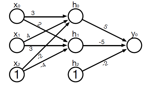
Your Turn

Put the returned weights and biases into the XOR neural network diagram and try to work out the output when the input is [0,0].

4.3.4. Inference (Forward Pass)¶

Instead of verifying it maually, we can test out our XOR model, with input [0,1] by called the model with the input. Note we do not call the forward function directly, instead we provide input to the model.

model(torch.tensor([0.,1.]).to(device))

tensor([0.9715], device='cuda:0', grad_fn=<SigmoidBackward>)

4.4. Logging the model training for Visualisation in TensorBoard¶

TensorBoard by TensorFlow is a very useful tool for visualising training progress and model architectures, despite being a competiting platform, PyTorch provides classes and methods for us to integrate it with our model.

TensorBoard can be loaded inside Jupyter notebooks, or can be started externally from a command line. Before we run TensorBoard, we need to change to the directory of your model code, and create a folder, e.g. runs to keep a log of the training progress.

The examples in this lab are running Tensorboard inside a notebook, but it is a good idea to run TensorBoard on the command line by giving the log directory. Assuming you are one level up the runs directory:

tensorboard --logdir runs

If successful, it will say that TensorBoard 2.6.0 at http://localhost:6006/ (Press CTRL+C to quit), copy and paste the URL to your browser to see TensorBoard in action.

%load_ext tensorboard

4.4.1. TensorBoard running in Jupyter Notebook¶

%tensorboard --logdir runs

4.4.2. SummaryWriter¶

It all starts with the creation of a SummaryWriter. TensorBoard to look for logs inside the runs folder, it only makes sense to actually log to that folder. Moreover, to be able to distinguish between different experiments or models, we should also specify a sub-folder: test.

If we do not specify any folder, TensorBoard will default to runs/CURRENT_DATETIME_HOSTNAME, which is not such a great name if you’d be looking for your experiment results in the future.

So, it is recommended to try to name it in a more meaningful way, like runs/test or runs/simple_linear_regression. It will then create a subfolder inside runs (the folder we specified when we started TensorBoard).

Even better, you should name it in a meaningful way and add datetime or a sequential number as a suffix, like runs/test_001 or runs/test_20200502172130, to avoid writing data of multiple runs into the same folder (we’ll see why this is bad in the add_scalars section below).

from torch.utils.tensorboard import SummaryWriter
writer = SummaryWriter('runs/test')

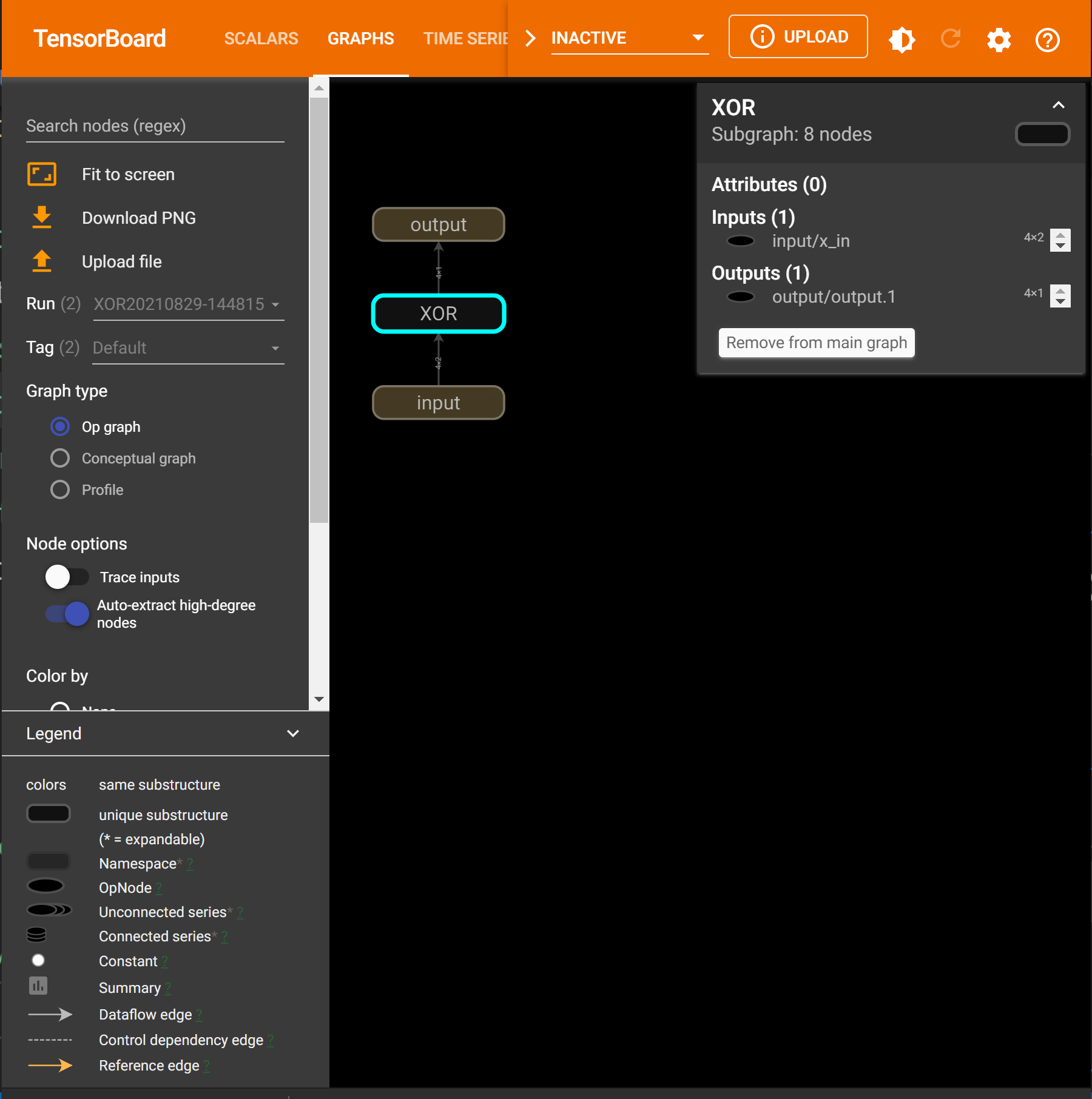
4.4.3. `add_graph`¶

It will produce an input-output graph that allows you to interactively inspect parameters, which is different from the TorchViz’s computation graph (a static visualisation - not interactive).

writer.add_graph(model, x_train_tensor)
%tensorboard --logdir runs

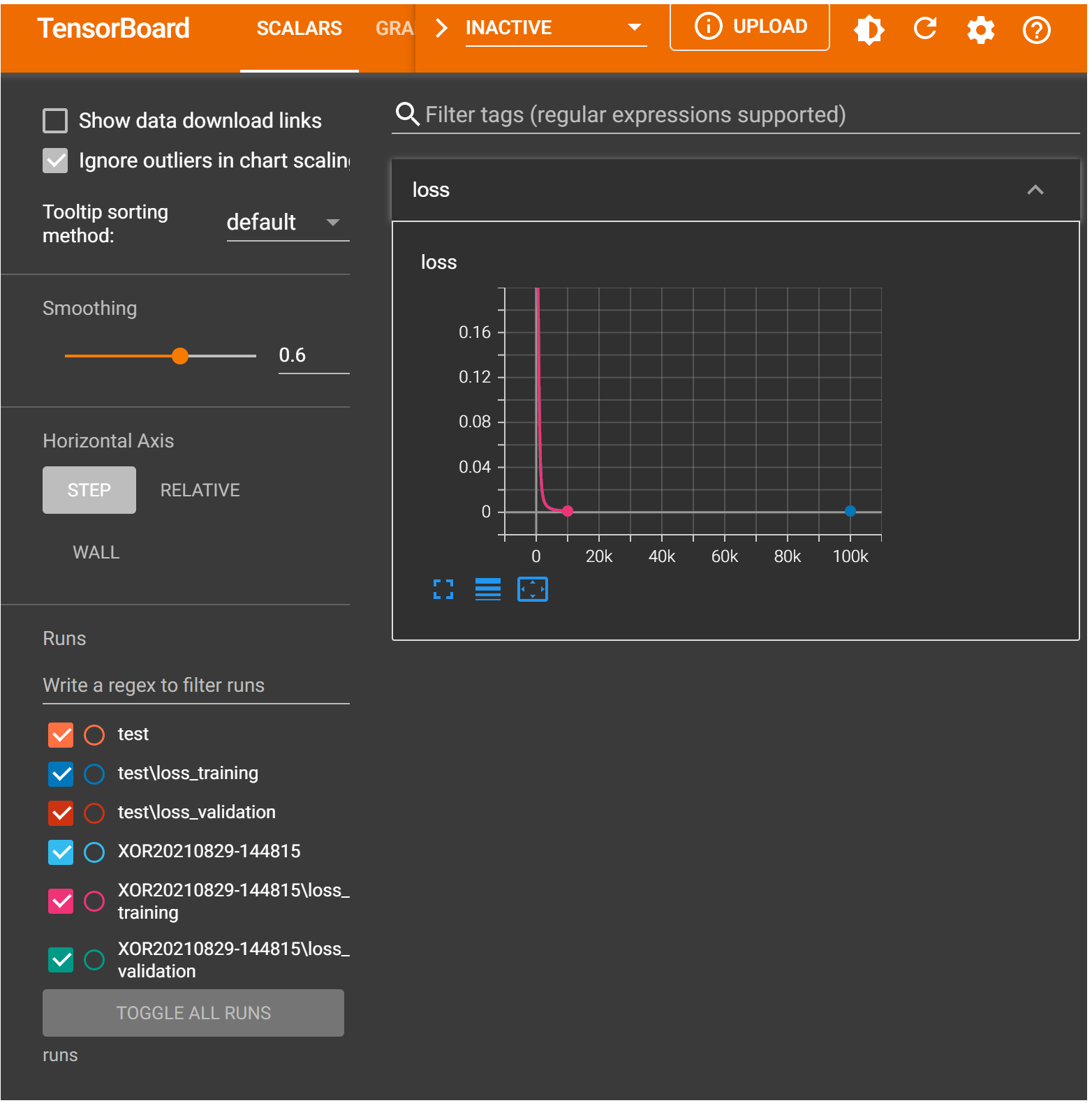
4.4.4. `add_scalar`¶

We can send the loss values to TensorBoard using the add_scalars method to send multiple scalar values at once, and it needs three arguments:

main_tag: the parent name of the tags or, the “group tag”
tag_scalar_dict: the dictionary containing the key: value pairs for the scalars you want to keep track of (can be training and validation losses)
global_step: step value, that is, the index you’re associating with the values you’re sending in the dictionary - the epoch comes to mind in our case, as losses are computed for each epoch

writer.add_scalars(main_tag='loss',
    tag_scalar_dict={'training': loss,
                    'validation': loss},
    global_step=epoch
)

If you run the code above after performing the model training, it will just send both loss values computed for the last epoch.

%tensorboard --logdir runs

from datetime import datetime
# Sets learning rate - this is "eta" ~ the "n" like
# Greek letter
lr = 0.1

# Step 0 - Initializes parameters "b" and "w" randomly
torch.manual_seed(42)
# Now we can create a model and send it at once to the device
model = XOR(2,1)
model = model.to(device)

# Defines a SGD optimizer to update the parameters
# (now retrieved directly from the model)
optimizer = optim.SGD(model.parameters(), lr=lr)

# Defines a MSE loss function
loss_fn = nn.MSELoss(reduction='mean')

# Tensorboard setup
writer = SummaryWriter('runs/XOR' + datetime.now().strftime("%Y%m%d-%H%M%S"))
writer.add_graph(model, x_train_tensor.to(device))

# Defines number of epochs
n_epochs = 10000

losses = []
val_losses = [] # note we did not use the validation data
for epoch in range(n_epochs):
    #for j in range(steps):
    model.train() # What is this?!?

    # Step 1 - Computes model's predicted output - forward pass
    # No more manual prediction!
    yhat = model(x_train_tensor)

    # Step 2 - Computes the loss
    loss = loss_fn(yhat, y_train_tensor)
    
    # Step 3 - Computes gradients for both "b" and "w" parameters
    loss.backward()

    # Step 4 - Updates parameters using gradients and
    # the learning rate
    optimizer.step()
    optimizer.zero_grad()
    if (epoch % 500 == 0):
        print("Epoch: {0}, Loss: {1}, ".
            format(epoch, loss.to("cpu").detach().numpy()))

    losses.append(loss)
    writer.add_scalars(main_tag='loss', 
                       tag_scalar_dict={'training': loss,
                                      'validation': loss},
                       global_step=epoch)

writer.close()                        

Epoch: 0, Loss: 0.27375736832618713, 
Epoch: 500, Loss: 0.2081705629825592, 
Epoch: 1000, Loss: 0.09176724404096603, 
Epoch: 1500, Loss: 0.03289078176021576, 
Epoch: 2000, Loss: 0.016263967379927635, 
Epoch: 2500, Loss: 0.009998900815844536, 
Epoch: 3000, Loss: 0.006978640332818031, 
Epoch: 3500, Loss: 0.005261328537017107, 
Epoch: 4000, Loss: 0.00416548689827323, 
Epoch: 4500, Loss: 0.0034290249459445477, 
Epoch: 5000, Loss: 0.002894176635891199, 
Epoch: 5500, Loss: 0.002497166395187378, 
Epoch: 6000, Loss: 0.0021936693228781223, 
Epoch: 6500, Loss: 0.0019435270223766565, 
Epoch: 7000, Loss: 0.0017444714903831482, 
Epoch: 7500, Loss: 0.0015824229922145605, 
Epoch: 8000, Loss: 0.001446553273126483, 
Epoch: 8500, Loss: 0.0013299942947924137, 
Epoch: 9000, Loss: 0.00122724543325603, 
Epoch: 9500, Loss: 0.0011413537431508303, 

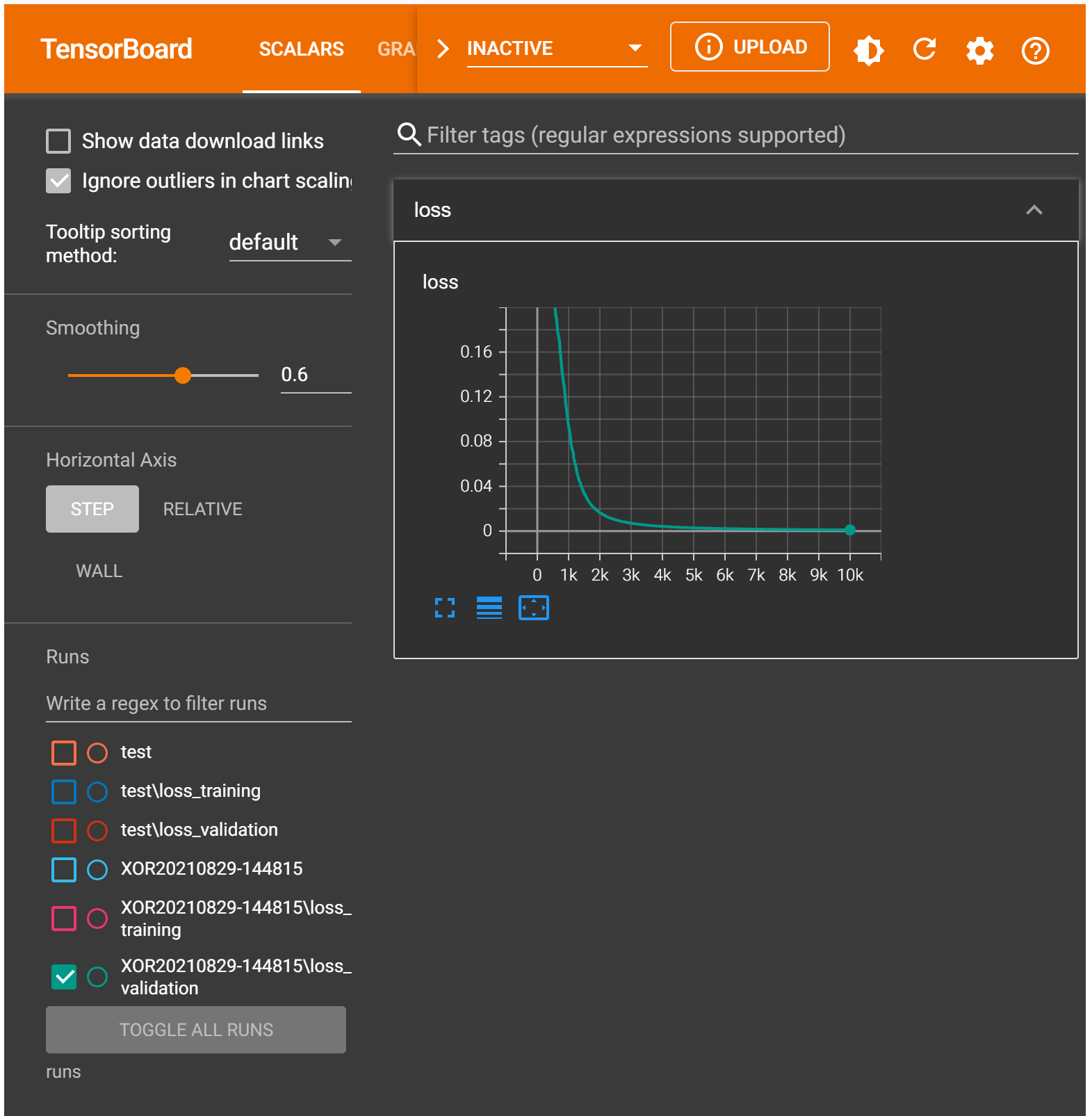
%tensorboard --logdir runs

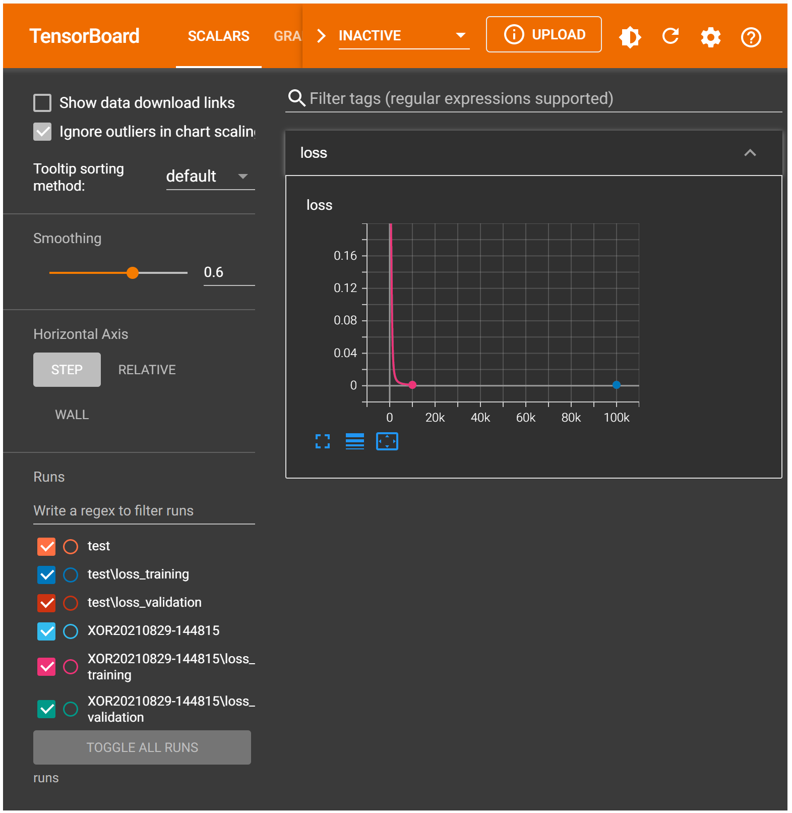
Note

In the TensorBoard logged run, we increased the learning rate and shortened the number of epochs. Play with these two parameters to see what you can get. Or change the loss function to BCE or BCEWithLogits to see how your training loss changes.

CITS4012 Natural Language Processing

4. Neural Networks in PyTorch¶

4.1. A neural network with one hidden layer¶

4.1.1. Defining the model class¶

4.1.2. Object Orientation in PyTorch¶

4.2. XOR Model¶

4.2.1. Obtain all model parameters using state_dict()¶

4.2.2. Model and Data need to be on the same device¶

4.3. Training XOR¶

4.3.1. Training Data Preparation¶

4.3.2. Hyperparameter setup¶

4.3.3. Training¶

4.3.4. Inference (Forward Pass)¶

4.4. Logging the model training for Visualisation in TensorBoard¶

4.4.1. TensorBoard running in Jupyter Notebook¶

4.4.2. SummaryWriter¶

4.4.3. add_graph¶

4.4.4. add_scalar¶

4.2.1. Obtain all model parameters using `state_dict()`¶

4.4.3. `add_graph`¶

4.4.4. `add_scalar`¶