1. Starting with NLTK¶

If you have installed nltk and have downloaded the data and models, you can skip this.

import nltk
nltk.download()

Downloading the NLTK Book Collection: browse the available packages using nltk.download(). The Collections tab on the downloader shows how the packages are grouped into sets, and you should select the line labeled book to obtain all data required for the examples and exercises in this book. It consists of about 30 compressed files requiring about 100Mb disk space. The full collection of data (i.e., all in the downloader) is nearly ten times this size (at the time of writing) and continues to expand.

Once the data is downloaded to your machine, you can load some of it using the Jupyter Notebook. The first step is to type a special command which tells the interpreter to load some texts for us to explore: from nltk.book import *. This says “from NLTK’s book module, load all items.” The book module contains all the data you will need as you read this chapter. After printing a welcome message, it loads the text of several books (this will take a few seconds). Here’s the command again, together with the output that you will see. Take care to get spelling and punctuation right.

from nltk.book import *

*** Introductory Examples for the NLTK Book ***
Loading text1, ..., text9 and sent1, ..., sent9
Type the name of the text or sentence to view it.
Type: 'texts()' or 'sents()' to list the materials.
text1: Moby Dick by Herman Melville 1851
text2: Sense and Sensibility by Jane Austen 1811
text3: The Book of Genesis
text4: Inaugural Address Corpus
text5: Chat Corpus
text6: Monty Python and the Holy Grail
text7: Wall Street Journal
text8: Personals Corpus
text9: The Man Who Was Thursday by G . K . Chesterton 1908

Any time we want to find out about these texts, we just have to enter their names at the Python prompt:

text1

<Text: Moby Dick by Herman Melville 1851>

text2

<Text: Sense and Sensibility by Jane Austen 1811>

Now that we have some data to work with, we’re ready to get started.

1.1. Searching Text¶

1.1.1. Concordance¶

There are many ways to examine the context of a text apart from simply reading it. A concordance view shows us every occurrence of a given word, together with some context. Here we look up the word monstrous in Moby Dick:

text1.concordance("monstrous")

Displaying 11 of 11 matches:
ong the former , one was of a most monstrous size . ... This came towards us , 
ON OF THE PSALMS . " Touching that monstrous bulk of the whale or ork we have r
ll over with a heathenish array of monstrous clubs and spears . Some were thick
d as you gazed , and wondered what monstrous cannibal and savage could ever hav
that has survived the flood ; most monstrous and most mountainous ! That Himmal
they might scout at Moby Dick as a monstrous fable , or still worse and more de
th of Radney .'" CHAPTER 55 Of the Monstrous Pictures of Whales . I shall ere l
ing Scenes . In connexion with the monstrous pictures of whales , I am strongly
ere to enter upon those still more monstrous stories of them which are to be fo
ght have been rummaged out of this monstrous cabinet there is no telling . But 
of Whale - Bones ; for Whales of a monstrous size are oftentimes cast up dead u

The first time you use a concordance on a particular text, it takes a few extra seconds to build an index so that subsequent searches are fast.

Your Turn

Try searching for other words,
You can also try searches on some of the other texts we have included. For example, search Sense and Sensibility for the word affection, using text2.concordance(“affection”).
Search the book of Genesis to find out how long some people lived, using text3.concordance("lived").
You could look at text4, the Inaugural Address Corpus, to see examples of English going back to 1789, and search for words like nation, terror, god to see how these words have been used differently over time.
We’ve also included text5, the NPS Chat Corpus: search this for unconventional words like im, ur, lol. (Note that this corpus is uncensored!)

Once you’ve spent a little while examining these texts, we hope you have a new sense of the richness and diversity of language.

1.1.2. Similar Words and Common Context¶

A concordance permits us to see words in context. For example, we saw that monstrous occurred in contexts such as the ___ pictures and a ___ size . What other words appear in a similar range of contexts? We can find out by using similar() function for the text object (e.g. text1) with the word (e.g. monstrous) as its argument:

text1.similar("monstrous")

true contemptible christian abundant few part mean careful puzzled
mystifying passing curious loving wise doleful gamesome singular
delightfully perilous fearless

text2.similar("monstrous")

very so exceedingly heartily a as good great extremely remarkably
sweet vast amazingly

Observe that we get different results for different texts. Austen uses this word quite differently from Melville; for her, monstrous has positive connotations, and sometimes functions as an intensifier like the word very.

The term common_contexts allows us to examine just the contexts that are shared by two or more words, such as monstrous and very. We have to enclose these words by square brackets as well as parentheses, and separate them with a comma:

text2.common_contexts(["monstrous", "very"])

am_glad a_pretty a_lucky is_pretty be_glad

Your Turn

Pick another pair of words and compare their usage in two different texts, using the similar() and common_contexts() functions.

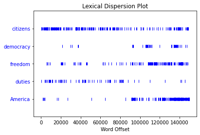
We have seen how to automatically detect that a particular word occurs in a text, and to display some words that appear in the same context. We can also determine the location of a word in the text: how many words from the beginning it appears. This positional information can be displayed using a dispersion plot. Each stripe represents an instance of a word, and each row represents the entire text. We can see the dispersion of words in text4 (Inaugural Address Corpus). You can produce this plot as shown below. You might like to try more words (e.g., liberty, constitution), and different texts. Can you predict the dispersion of a word before you view it? As before, take care to get the quotes, commas, brackets and parentheses exactly right.

text4.dispersion_plot(["citizens", "democracy", "freedom", "duties", "America"])

Important

You need to have Python’s NumPy and Matplotlib packages installed in order to produce the graphical plots used in this book. Please see http://nltk.org/ for installation instructions.

You can also plot the frequency of word usage through time using https://books.google.com/ngrams

1.1.3. Generating Text¶

Now, just for fun, let’s try generating some random text in the various styles we have just seen. To do this, we type the name of the text followed by the term generate. (We need to include the parentheses, but there’s nothing that goes between them.)

text3.generate()

Building ngram index...

laid by her , and said unto Cain , Where art thou , and said , Go to ,
I will not do it for ten ' s sons ; we dreamed each man according to
their generatio the firstborn said unto Laban , Because I said , Nay ,
but Sarah shall her name be . , duke Elah , duke Shobal , and Akan .
and looked upon my affliction . Bashemath Ishmael ' s blood , but Isra
for as a prince hast thou found of all the cattle in the valley , and
the wo The

"laid by her , and said unto Cain , Where art thou , and said , Go to ,\nI will not do it for ten ' s sons ; we dreamed each man according to\ntheir generatio the firstborn said unto Laban , Because I said , Nay ,\nbut Sarah shall her name be . , duke Elah , duke Shobal , and Akan .\nand looked upon my affliction . Bashemath Ishmael ' s blood , but Isra\nfor as a prince hast thou found of all the cattle in the valley , and\nthe wo The"

1.2. Counting Vocabulary¶

The most obvious fact about texts that emerges from the preceding examples is that they differ in the vocabulary they use. In this section we will see how to use the computer to count the words in a text in a variety of useful ways. Test your understanding by modifying the examples, and trying the exercises at the end of this lab.

1.2.1. Text Size vs. Vocabulary Size¶

Let’s begin by finding out the length of a text from start to finish, in terms of the words and punctuation symbols that appear. We use the term len to get the length of something, which we’ll apply here to the book of Genesis:

len(text3)

So Genesis has 44,764 words and punctuation symbols, or “tokens.” A token is the technical name for a sequence of characters — such as hairy, his, or :) — that we want to treat as a group. When we count the number of tokens in a text, say, the phrase to be or not to be, we are counting occurrences of these sequences. Thus, in our example phrase there are two occurrences of to, two of be, and one each of or and not. But there are only four distinct vocabulary items in this phrase.

Your Turn

How many distinct words does the book of Genesis contain?

To work this out in Python, we have to pose the question slightly differently. The vocabulary of a text is just the set of tokens that it uses, since in a set, all duplicates are collapsed together. In Python we can obtain the vocabulary items of text3 with the command: set(text3). When you do this, many screens of words will fly past. Now try the following. By wrapping sorted() around the Python expression set(text3), we obtain a sorted list of vocabulary items, beginning with various punctuation symbols and continuing with words starting with A. All capitalized words precede lowercase words. [:20] will list the first 20 tokens, not including the token indexed by 20.

sorted(set(text3)) [:20]

['!',
 "'",
 '(',
 ')',
 ',',
 ',)',
 '.',
 '.)',
 ':',
 ';',
 ';)',
 '?',
 '?)',
 'A',
 'Abel',
 'Abelmizraim',
 'Abidah',
 'Abide',
 'Abimael',
 'Abimelech']

len(set(text3))

We discover the size of the vocabulary indirectly, by asking for the number of items in the set, and again we can use len to obtain this number. Although it has 44,764 tokens, this book has only 2,789 distinct words, or “word types.” A word type is the form or spelling of the word independently of its specific occurrences in a text — that is, the word considered as a unique item of vocabulary. Our count of 2,789 items will include punctuation symbols, so we will generally call these unique items types instead of word types.

1.2.2. Lexical Richness¶

Now, let’s calculate a measure of the lexical richness of the text. The next example shows us that the number of distinct words is just 6% of the total number of words, or equivalently that each word is used 16 times on average.

len(set(text3)) / len(text3)

0.06230453042623537

1.2.3. Word Freqency¶

Next, let’s focus on particular words. We can count how often a word occurs in a text, and compute what percentage of the text is taken up by a specific word:

# raw count
text3.count("smote")

# percentage frequency
100 * text4.count('a') / len(text4)

1.457973123627309

Your Turn

How many times does the word lol appear in text5? How much is this as a percentage of the total number of words in this text?

Your Turn

You may want to repeat such calculations on several texts, but it is tedious to keep retyping the formula. Instead, you can come up with your own name for a task, like “lexical_diversity” or “tf” (for term frequency), and associate it with a block of code. Now you only have to type a short name instead of one or more complete lines of Python code, and you can re-use it as often as you like. The block of code that does a task for us is called a function, and we define a short name for our function with the keyword def. The next example shows how to define two new functions, lexical_diversity() and tf():

def lexical_diversity(text):
    return len(set(text)) / len(text)

def tf(text, token):
    count = text.count(token)
    total = len(text)
    return 100 * count / total

In the definition of lexical_diversity(), we specify a parameter named text . This parameter is a “placeholder” for the actual text whose lexical diversity we want to compute, and reoccurs in the block of code that will run when the function is used. Similarly, tf() is defined to take two parameters, named text and token.

Once Python knows that lexical_diversity() and tf() are the names for specific blocks of code, we can go ahead and use these functions:

lexical_diversity(text3)

0.06230453042623537

tf(text4, 'a')

1.457973123627309

To recap, we use or call a function such as lexical_diversity() by typing its name, followed by an open parenthesis, the name of the text, and then a close parenthesis. These parentheses will show up often; their role is to separate the name of a task — such as lexical_diversity() — from the data that the task is to be performed on — such as text3. The data value that we place in the parentheses when we call a function is an argument to the function.

You have already encountered several functions in this lab, such as len(), set(), and sorted(). By convention, we will always add an empty pair of parentheses after a function name, as in len(), just to make clear that what we are talking about is a function rather than some other kind of Python expression. Functions are an important concept in programming, you should consider refactoring frequently reusable blocks of code into functions.

Later we’ll see how to use functions when tabulating data. Each row of the table will involve the same computation but with different data, and we’ll do this repetitive work using a function.

Table 1.1 Lexical Diversity of Various Genres in the Brown Corpus¶
Genre	Tokens	Types	Lexical diversity
skill and hobbies	82345	11935	0.145
humor	21695	5017	0.231
fiction: science	14470	3233	0.223
press: reportage	100554	14394	0.143
fiction: romance	70022	8452	0.121
religion	39399	6373	0.162

CITS4012 Natural Language Processing

1. Starting with NLTK¶

1.1. Searching Text¶

1.1.1. Concordance¶

1.1.2. Similar Words and Common Context¶

1.1.3. Generating Text¶

1.2. Counting Vocabulary¶

1.2.1. Text Size vs. Vocabulary Size¶

1.2.2. Lexical Richness¶

1.2.3. Word Freqency¶