3. Convolution Basics¶

3.1. Convolution in Raw Numpy Code¶

There is one image, one channel, six by six pixels in size (shape $1\times 1\times 1 \times 6 \times 6). There is one filter, one channel, three by three pixels in size.

import numpy as np

single = np.array(
    [[[[5, 0, 8, 7, 8, 1],
    [1, 9, 5, 0, 7, 7],
    [6, 0, 2, 4, 6, 6],
    [9, 7, 6, 6, 8, 4],
    [8, 3, 8, 5, 1, 3],
    [7, 2, 7, 0, 1, 0]]]]
)
single.shape

(1, 1, 6, 6)

filter = np.array(
    [[[[0, 0, 0],
    [0, 1, 0],
    [0, 0, 0]]]]
    )
filter.shape

(1, 1, 3, 3)

region = single[:, :, 0:3, 0:3]
filtered_region = region * filter
total = filtered_region.sum()
total

new_region = single[:, :, 0:3, (0+1):(3+1)]

new_filtered_region = new_region * filter
new_total = new_filtered_region.sum()
new_total

last_horizontal_region = single[:, :, 0:3, (0+4):(3+4)]

last_horizontal_region * filter

---------------------------------------------------------------------------
ValueError                                Traceback (most recent call last)
~\AppData\Local\Temp/ipykernel_10920/1958888837.py in <module>
----> 1 last_horizontal_region * filter

ValueError: operands could not be broadcast together with shapes (1,1,3,2) (1,1,3,3) 

last_horizontal_region = single[:, :, 0:3, (0+4):(3+4)]

Applying a filter always produces a single value, the reduction is equal to the filter size minus one when stride is 1. For example, the above matrix is $6\times 6$, the filter size is $3 \times 3$, the reduction is $3-1=2$, the the resulting matrix is $4 \times 4$.

How do we generalise this to a $n \times m$ matrix, with a filter size $k \times l$ and a stride $d$. The shape of the newly reduced matrix is then:

\[ h \times w = n - (k-1) - (d-1) \times m - (l-1) - (d-1)\]

Your Turn

Based on the code above, write a function conv() that takes Arguments: input - a matrix to be converted
filter - a filter matrix stride - the number of places to move during convolution Returns: result - the resulting matrix after convolution

Make sure you take the border conditions into account.

def conv(input, filter, stride):
    # Setting up
    m, n = input.shape[2:4]
    k, l = filter.shape[2:4]
    result = np.zeros([1,1,(m-(k-1))//stride, (n-(l-1))//stride])
    h, w = result.shape[2:4]
    print(result.shape)
    row_idx = 0 # keep track of the row index of the output
    col_idx = 0 # keep track of the column index of the output
    for i in range(0, n, stride):
        for j in range(0, m, stride):
            if((i+k)<=n and (j+l)<=m and col_idx<w and row_idx<h ):
                result[:,:,row_idx,col_idx] = (input[:, :, i:i+k, j:j+l]*filter).sum()
                col_idx = col_idx + 1
        row_idx = row_idx + 1 
        col_idx = 0     
    return result            

conv(single, filter, 1)

(1, 1, 4, 4)

array([[[[9., 5., 0., 7.],
         [0., 2., 4., 6.],
         [7., 6., 6., 8.],
         [3., 8., 5., 1.]]]])

conv(single, filter, 2)

(1, 1, 2, 2)

array([[[[9., 0.],
         [7., 6.]]]])

3.2. Convolving in PyTorch¶

kernel and filter are often used interchangably to refer to the matrix that will be applied over the original input matrix.

Just like the activation functions and loss functions we’ve seen in earlier labs, convolutions also come in two flavors: functional and module. There is a fundamental difference between the two, though: the functional convolution takes the kernel/filter as an argument while the module has weights to represent the kernel/filter. Let’s use the functional convolution, F.conv2d, to apply the filter to our input matrix (notice we’re using stride=1 since we moved the region around one pixel at a time.

Note

We need to convert Numpy arrays into Torch Tensors before we can make use the F.conv2d function.

import torch
import torch.nn.functional as F
image = torch.as_tensor(single).float()
kernel = torch.as_tensor(filter).float()
convolved = F.conv2d(image, kernel, stride=1)
convolved

tensor([[[[9., 5., 0., 7.],
          [0., 2., 4., 6.],
          [7., 6., 6., 8.],
          [3., 8., 5., 1.]]]])

Now, let’s turn our attention to PyTorch’s convolution module, nn.Conv2d. It has many arguments, let’s focus on the first four of them:

in_channels: number of channels of the input image
out_channels: number of channels produced by the convolution
kernel_size: size of the (square) convolution filter/kernel
stride: the size of the movement of the selected region

Important

First, there is no argument for the kernel/filter itself, there is only a kernel_size argument. This is because the actual filter is learned through training rather than specified.
Second, it is possible to produce multiple channels as output. It simply means the module is going to learn multiple filters. Each filter is going to produce a different result, which is being called a channel here.

For a single channel matrix (you can think of 2D matrices are images) as input, and applying one filter (size three by three) to it, moving one pixel at a time, resulting in one output/channel. This is what it looks like in nn.Conv2d code:

import torch.nn as nn
conv = nn.Conv2d(in_channels=1, out_channels=1, kernel_size=3, stride=1)
conv(image)

tensor([[[[-1.0575, -2.6052, -2.2154, -1.7589],
          [ 1.7594,  0.5861,  1.2595,  0.6742],
          [ 1.0704,  1.4473,  1.1077, -2.0348],
          [-1.6991, -1.5751, -1.4593, -3.0604]]]],
       grad_fn=<ThnnConv2DBackward>)

Important

These results are randomly initalised weights representing the kernel/filter. Yours will be different from this.

This is the whole point of the convolutional module: it will learn the kernel/filter on its own. In traditional computer vision, people would develop different filters for different purposes: blurring, sharpening, edge detection, and so on. But, instead of being clever and trying to manually devise a filter that does the trick for a given problem, why not outsource the filter definition to the neural network as well? This way the network will come up with filters that highlight features that are relevant to the task at hand.

Note

The resulting matrix shows a grad_fn attribute now: it will be used to compute gradients so the network can actually learn how to change the weights representing the filter.

Your Turn

Try changing the output channels to 2, and see how many filters have been randomly initialised.

3.2.1. Force to use a pre-defined filter¶

We can also force a convolutional module to use a particular filter by setting its weights.

Important

Setting the weights is a strictly no-gradient operation, so you should always use the no_grad context manager.

with torch.no_grad():
    conv.weight[0] = kernel
    conv.bias[0] = 0 

conv(image)    

tensor([[[[9., 5., 0., 7.],
          [0., 2., 4., 6.],
          [7., 6., 6., 8.],
          [3., 8., 5., 1.]]]], grad_fn=<ThnnConv2DBackward>)

3.3. Key hyperparameters in convolution¶

3.3.1. Dilation¶

Instead of a contiguous kernel, dilation controls the number of rows and columns to skip when the convolutional kernel is applied to the input matrix. In the code below, a dilation of two stretch the $2\time 2$ kernel into a holed $3\times 3$ kernel. The shape of the output feature map is therefore $4\times 4$.

conv_dilated = nn.Conv2d(in_channels=1, out_channels=1, 
          kernel_size=2, dilation=2, bias=False, stride=1)
conv_dilated(image)  # [1x1x6x6] tensor as input        

tensor([[[[ 2.0450, -0.8075,  2.1801,  1.3727],
          [-1.0471,  2.2050,  0.2247, -0.7972],
          [ 0.4034, -1.2558,  0.9169,  1.2028],
          [ 2.2282,  3.4014,  2.7813,  2.8520]]]],
       grad_fn=<SlowConvDilated2DBackward>)

3.3.2. Padding¶

By adding columns and rows of zeros around it, we expand the input image such that the gray region starts centered in the actual top left corner of the input image. This simple trick can be used to preserve the original size of the image. In code, as usual, PyTorch gives us two options: functional (F.pad) and module (nn.ConstantPad2d). Let’s start with the module version this time:

constant_padder = nn.ConstantPad2d(padding=1, value=0)
constant_padder(image)

tensor([[[[0., 0., 0., 0., 0., 0., 0., 0.],
          [0., 5., 0., 8., 7., 8., 1., 0.],
          [0., 1., 9., 5., 0., 7., 7., 0.],
          [0., 6., 0., 2., 4., 6., 6., 0.],
          [0., 9., 7., 6., 6., 8., 4., 0.],
          [0., 8., 3., 8., 5., 1., 3., 0.],
          [0., 7., 2., 7., 0., 1., 0., 0.],
          [0., 0., 0., 0., 0., 0., 0., 0.]]]])

One can also do asymmetric padding, by specifying a tuple in the padding argument representing (left, right, top, bottom). So, if we were to stuff our image on left and right sides only, the argument would go like this: (1, 1, 0, 0).

padded = F.pad(image, pad=(1, 1, 1, 1), mode='constant', value=0)
padded

tensor([[[[0., 0., 0., 0., 0., 0., 0., 0.],
          [0., 5., 0., 8., 7., 8., 1., 0.],
          [0., 1., 9., 5., 0., 7., 7., 0.],
          [0., 6., 0., 2., 4., 6., 6., 0.],
          [0., 9., 7., 6., 6., 8., 4., 0.],
          [0., 8., 3., 8., 5., 1., 3., 0.],
          [0., 7., 2., 7., 0., 1., 0., 0.],
          [0., 0., 0., 0., 0., 0., 0., 0.]]]])

There are three other modes: replicate, reflect, and circular.

Three Modes of Paddings

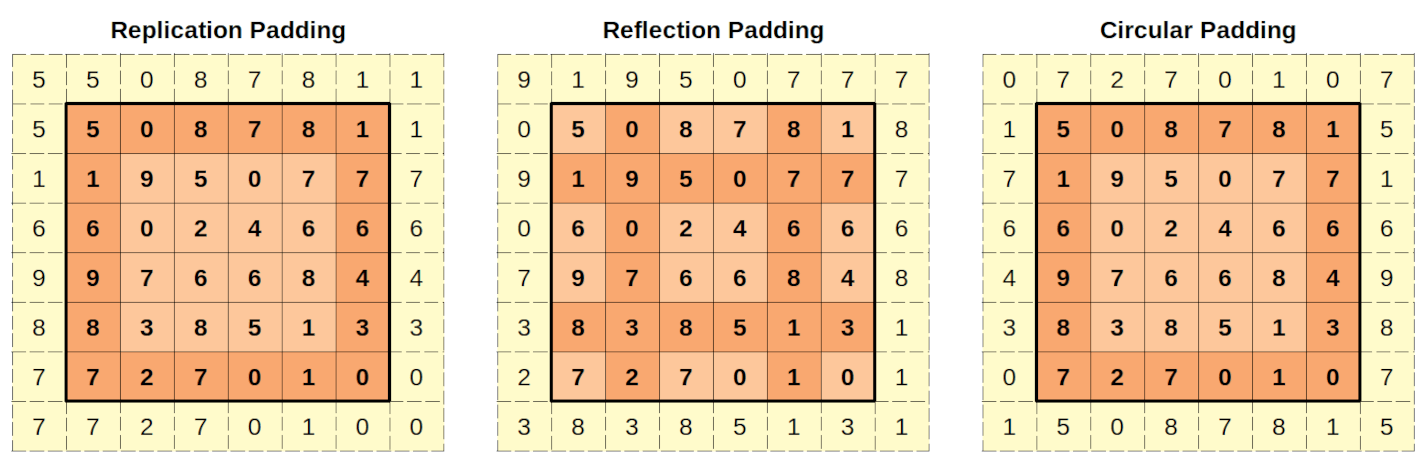
3.3.2.1. Replication Padding¶

In the replication padding, the padded pixels will have the same value as the closest real pixel. The padded corners will have the same value as the real corners. The other columns (left and right) and rows (top and bottom) will replicate the corresponding values of the original image. The values used in the replication are in a darker shade of orange.

In PyTorch, one can use the functional form F.pad with mode="replicate", or use the module version nn.ReplicationPad2d:

replication_padder = nn.ReplicationPad2d(padding=1)
replication_padder(image)

tensor([[[[5., 5., 0., 8., 7., 8., 1., 1.],
          [5., 5., 0., 8., 7., 8., 1., 1.],
          [1., 1., 9., 5., 0., 7., 7., 7.],
          [6., 6., 0., 2., 4., 6., 6., 6.],
          [9., 9., 7., 6., 6., 8., 4., 4.],
          [8., 8., 3., 8., 5., 1., 3., 3.],
          [7., 7., 2., 7., 0., 1., 0., 0.],
          [7., 7., 2., 7., 0., 1., 0., 0.]]]])

F.pad(image, pad=(1, 1, 1, 1), mode='replicate')

tensor([[[[5., 5., 0., 8., 7., 8., 1., 1.],
          [5., 5., 0., 8., 7., 8., 1., 1.],
          [1., 1., 9., 5., 0., 7., 7., 7.],
          [6., 6., 0., 2., 4., 6., 6., 6.],
          [9., 9., 7., 6., 6., 8., 4., 4.],
          [8., 8., 3., 8., 5., 1., 3., 3.],
          [7., 7., 2., 7., 0., 1., 0., 0.],
          [7., 7., 2., 7., 0., 1., 0., 0.]]]])

3.3.2.2. Reflection Padding¶

In the reflection padding, the outer columns and rows are used as axes for the reflection. So, the left padded column (forget about the corners for now) will reflect the second column (since the first column is the axis of reflection). The same reasoning goes for the right padded column. Similarly, the top padded row will reflect the second row (since the first row is the axis of reflection), and the same reasoning goes for the bottom padded row. The values used in the reflection are in a darker shade of orange. The corners will have the same values as the intersection of the reflected rows and columns of the original image, or the diagnol value when the original corners are used as a reflection point.

In PyTorch, you can use the functional form F.pad with mode="reflect", or use the module version nn.ReflectionPad2d.

reflection_padder = nn.ReflectionPad2d(padding=1)
reflection_padder(image)

tensor([[[[9., 1., 9., 5., 0., 7., 7., 7.],
          [0., 5., 0., 8., 7., 8., 1., 8.],
          [9., 1., 9., 5., 0., 7., 7., 7.],
          [0., 6., 0., 2., 4., 6., 6., 6.],
          [7., 9., 7., 6., 6., 8., 4., 8.],
          [3., 8., 3., 8., 5., 1., 3., 1.],
          [2., 7., 2., 7., 0., 1., 0., 1.],
          [3., 8., 3., 8., 5., 1., 3., 1.]]]])

F.pad(image, pad=(1, 1, 1, 1), mode='reflect')

tensor([[[[9., 1., 9., 5., 0., 7., 7., 7.],
          [0., 5., 0., 8., 7., 8., 1., 8.],
          [9., 1., 9., 5., 0., 7., 7., 7.],
          [0., 6., 0., 2., 4., 6., 6., 6.],
          [7., 9., 7., 6., 6., 8., 4., 8.],
          [3., 8., 3., 8., 5., 1., 3., 1.],
          [2., 7., 2., 7., 0., 1., 0., 1.],
          [3., 8., 3., 8., 5., 1., 3., 1.]]]])

3.3.2.3. Circular Padding¶

In the circular padding, the left-most (right-most) column gets copied as the right (left) padded column (forget about the corners for now too). Similarly, the topmost (bottom-most) row gets copied as the bottom (top) padded row. The corners will receive the values of the diametrically opposed corner: the top-left padded pixel receives the value of the bottom-right corner of the original image. Once again, the values used in the padding are in a darker shade of orange.

In PyTorch, you must use the functional form F.pad with mode="circular" since there is no module version of the circular padding (at time of writing):

F.pad(image, pad=(1, 1, 1, 1), mode='circular')

tensor([[[[0., 7., 2., 7., 0., 1., 0., 7.],
          [1., 5., 0., 8., 7., 8., 1., 5.],
          [7., 1., 9., 5., 0., 7., 7., 1.],
          [6., 6., 0., 2., 4., 6., 6., 6.],
          [4., 9., 7., 6., 6., 8., 4., 9.],
          [3., 8., 3., 8., 5., 1., 3., 8.],
          [0., 7., 2., 7., 0., 1., 0., 7.],
          [1., 5., 0., 8., 7., 8., 1., 5.]]]])

3.3.3. Pooling to Shrink Images¶

Another way of shrinking images is to use pooling. It is different from the former operations: it splits the image into tiny chunks, performs an operation on each chunk (that yields a single value), and puts the chunks together as the resulting image. For example, a $6\times 6$ image can be reduced to $3\times 3$ by splitting the original image to 9 chunks.

In PyTorch, as usual, we have both forms: F.max_pool2d and nn.MaxPool2d.

pooled = F.max_pool2d(padded, kernel_size=2)
pooled

C:\ProgramData\Anaconda3\envs\cits4012\lib\site-packages\torch\nn\functional.py:718: UserWarning: Named tensors and all their associated APIs are an experimental feature and subject to change. Please do not use them for anything important until they are released as stable. (Triggered internally at  ..\c10/core/TensorImpl.h:1156.)
  return torch.max_pool2d(input, kernel_size, stride, padding, dilation, ceil_mode)

tensor([[[[5., 8., 8., 1.],
          [6., 9., 7., 7.],
          [9., 8., 8., 4.],
          [7., 7., 1., 0.]]]])

A pooling kernel of two-by-two results in an image whose dimensions are half of the original.
A pooling kernel of three-by-three makes the resulting image one third the size of the original, and so on.

Important

only full chunks count: if we try a kernel of five-by-five in our eight-by-eight image, only one chunk fits, and the resulting image would have a single pixel.

maxpool5 = nn.MaxPool2d(kernel_size=5)
pooled5 = maxpool5(padded)
pooled5

tensor([[[[9.]]]])

Besides max-pooling, average pooling is also fairly common. As the name suggests, it will output the average pixel value for each chunk. In PyTorch, we have F.avg_pool2d and nn.AvgPool2d.

You can also use a stride greater than 1 just like applying a convolution kernel:

padded

tensor([[[[0., 0., 0., 0., 0., 0., 0., 0.],
          [0., 5., 0., 8., 7., 8., 1., 0.],
          [0., 1., 9., 5., 0., 7., 7., 0.],
          [0., 6., 0., 2., 4., 6., 6., 0.],
          [0., 9., 7., 6., 6., 8., 4., 0.],
          [0., 8., 3., 8., 5., 1., 3., 0.],
          [0., 7., 2., 7., 0., 1., 0., 0.],
          [0., 0., 0., 0., 0., 0., 0., 0.]]]])

F.max_pool2d(padded, kernel_size=2, stride=2)

tensor([[[[5., 8., 8., 1.],
          [6., 9., 7., 7.],
          [9., 8., 8., 4.],
          [7., 7., 1., 0.]]]])

3.3.4. Flatterning¶

It simply flattens a tensor, by appending the values of each row to its previous row. It has a module version nn.Flatten(). There is no functional version of it, as it can achieved by the view() function.

pooled

tensor([[[[5., 8., 8., 1.],
          [6., 9., 7., 7.],
          [9., 8., 8., 4.],
          [7., 7., 1., 0.]]]])

flatterned = nn.Flatten()(pooled)
flatterned

tensor([[5., 8., 8., 1., 6., 9., 7., 7., 9., 8., 8., 4., 7., 7., 1., 0.]])

pooled.view(1,-1)

tensor([[5., 8., 8., 1., 6., 9., 7., 7., 9., 8., 8., 4., 7., 7., 1., 0.]])

3.4. 1D Convolution¶

Give a sequence of daily temperature readings, let’s use a window (filter) of size five, like in the figure below. In its first step, the window is over days one to five. In the next step, since it can only move to the right, it will be over days two to six. The size of our movement to the right is, the stride.

Now, let’s assign the same value (0.2 = $\frac{1}{5}$) for every weight in our filter and use PyTorch’s F.conv1d to convolve the filter with our sequence (the shape is the NCL: the Number of sequences, the number of Channels and the Length of the sequence.):

import torch.nn.functional as F
import numpy as np
import torch

temperatures = np.array([5, 11, 15, 6, 5, 3, 3, 0, 0, 3, 4, 2, 1])
size = 5
weight = torch.ones(size) * 0.2
F.conv1d(torch.as_tensor(temperatures).float().view(1, 1, -1),
         weight=weight.view(1, 1, -1))

tensor([[[8.4000, 8.0000, 6.4000, 3.4000, 2.2000, 1.8000, 2.0000, 1.8000,
          2.0000]]])

This is a moving average, as we have the same weight ($\frac{1}{window\_size}$) for the weighted sum.

weight

tensor([0.2000, 0.2000, 0.2000, 0.2000, 0.2000])

import torch.nn as nn
torch.manual_seed(17)
conv_seq = nn.Conv1d(in_channels=10, out_channels=100,
    kernel_size=2, bias=False)
conv_seq.weight, conv_seq.weight.shape

(Parameter containing:
 tensor([[[-0.0294,  0.0157],
          [ 0.1477, -0.1682],
          [-0.2105,  0.0221],
          ...,
          [-0.0651, -0.1261],
          [-0.2236, -0.1607],
          [ 0.0448,  0.0294]],
 
         [[-0.1812, -0.1802],
          [-0.0575, -0.2116],
          [-0.1365,  0.1271],
          ...,
          [ 0.2072,  0.0923],
          [ 0.1267,  0.1031],
          [-0.0246, -0.0949]],
 
         [[-0.1262, -0.1012],
          [ 0.1101, -0.0824],
          [-0.0500,  0.1758],
          ...,
          [-0.1602,  0.0048],
          [ 0.1420, -0.1564],
          [ 0.1490, -0.1395]],
 
         ...,
 
         [[ 0.1480, -0.1971],
          [-0.1273,  0.0995],
          [-0.0726, -0.1250],
          ...,
          [ 0.1296,  0.1590],
          [-0.0313,  0.1204],
          [-0.1540, -0.0166]],
 
         [[ 0.1235,  0.2034],
          [ 0.0404, -0.0861],
          [ 0.0900, -0.1462],
          ...,
          [ 0.0307,  0.1345],
          [-0.1840, -0.1889],
          [-0.0731,  0.0381]],
 
         [[ 0.1546, -0.0249],
          [-0.1551,  0.0903],
          [-0.0173, -0.1090],
          ...,
          [ 0.1704,  0.2202],
          [-0.2147,  0.2092],
          [-0.1115,  0.1248]]], requires_grad=True),
 torch.Size([100, 10, 2]))

CITS4012 Natural Language Processing

3. Convolution Basics¶

3.1. Convolution in Raw Numpy Code¶

3.2. Convolving in PyTorch¶

3.2.1. Force to use a pre-defined filter¶

3.3. Key hyperparameters in convolution¶

3.3.1. Dilation¶

3.3.2. Padding¶

3.3.2.1. Replication Padding¶

3.3.2.2. Reflection Padding¶

3.3.2.3. Circular Padding¶

3.3.3. Pooling to Shrink Images¶

3.3.4. Flatterning¶

3.4. 1D Convolution¶